How to Parallelize a Transformer for Training
Part 5 of How To Scale Your Model (Part 4: Transformers | Part 6: Training LLaMA)
Here we discuss four main parallelism schemes used during LLM training: data parallelism, fully-sharded data parallelism (FSDP), tensor parallelism, and pipeline parallelism. For each, we calculate at what point we become bottlenecked by communication.
What Do We Mean By Scaling?
The goal of “model scaling” is to be able to increase the number of chips used for training or inference while achieving a proportional, linear increase in throughput (we call this strong scaling). While performance on a single chip depends on the trade-off between memory bandwidth and FLOPs, performance at the cluster level depends on hiding inter-chip communication by overlapping it with useful FLOPs. This is non-trivial, because increasing the number of chips increases the communication load while reducing the amount of per-device computation we can use to hide it. As we saw in Section 3, sharded matrix multiplications often require expensive AllGathers or ReduceScatters that can block the TPUs from doing useful work. The goal of this section is to find out when these become too expensive.
In this section, we’ll discuss four common parallelism schemes: (pure) data parallelism, fully-sharded data parallelism (FSDP / ZeRO sharding), tensor parallelism (also known as model parallelism), and (briefly) pipeline parallelism. For each, we’ll show what communication cost we incur and at what point that cost starts to bottleneck our compute cost.
We’ll use the following notation to simplify calculations throughout this section.
| Notation | Meaning (model parameters) |
|---|---|
| D | dmodel (the hidden dimension/residual stream dim) |
| F | dff (the feed-forward dimension) |
| B | Batch dimension (number of tokens in the batch; total, not per-device) |
| T | Sequence length |
| L | Number of layers in the model |
| Notation | Meaning (hardware characteristic) |
|---|---|
| C | FLOPS/s per chip |
| W | Network bandwidth (bidirectional, often subscripted as e.g. $W_{\text{ici}}$ or $W_{\text{dcn}}$) |
| X | Number of chips along mesh axis X |
| Y | Number of chips along an alternate mesh axis, labeled Y |
| Z | Number of chips along a third mesh axis, labeled Z |
For simplicity’s sake, we’ll approximate a Transformer as a stack of MLP blocks — attention is a comparatively small fraction of the FLOPs for larger models as we saw in Section 4. We will also ignore the gating matmul, leaving us with the following simple structure for each layer:
bf16[D, F] (up-projection) and Wout: bf16[F, D] (down-projection) with an input In: bf16[B, D].Here’s the full algorithm for our little Transformer with no parallelism.
Forward pass: need to compute Loss[B]
- Tmp[B, F] = In[B, D] *D Win[D, F]
- Out[B, D] = Tmp[B, F] *F Wout[F, D]
- Loss[B] = …
Backward pass: need to compute dWout[F, D], dWin[D, F]
- dOut[B, D] = …
- dWout[F, D] = Tmp[B, F] *B dOut[B, D]
- dTmp[B, F] = dOut[B, D] *D Wout[F, D]
- dWin[D, F] = In[B, D] *B dTmp[B, F]
- dIn[B, D] = dTmp[B, F] *F Win[D, F] (needed for previous layers)
We provide this for comparison to the algorithms with communication added.
Here are the 4 parallelism schemes we will discuss. Each scheme can be thought of as uniquely defined by a sharding for In, Win, Wout, and Out in the above diagram.
1. Data parallelism: activations sharded along batch, parameters and optimizer state are replicated on each device. Communication only occurs during the backwards pass.
\[\text{In}[B_X, D] \cdot_D W_\text{in}[D, F] \cdot_F W_\text{out}[F, D] \rightarrow \text{Out}[B_X, D]\]2. Fully-sharded data parallelism (FSDP or ZeRO-3): activations sharded along batch (like pure data parallelism), parameters sharded along same mesh axis and AllGathered just-in-time before use in forward pass. Optimizer state also sharded along batch. Reduces duplicated memory.
\[\text{In}[B_X, D] \cdot_D W_\text{in}[D_X, F] \cdot_F W_\text{out}[F, D_X] \rightarrow \text{Out}[B_X, D]\]3. Tensor parallelism (also called Megatron sharding or model parallelism): activations sharded along D ($d_\text{model}$), parameters sharded along F ($d_{ff}$). AllGather and ReduceScatter activations before and after each block. Compatible with FSDP.
\[\text{In}[B, D_Y] \cdot_D W_\text{in}[D, F_Y] \cdot_F W_\text{out}[F_Y, D] \rightarrow \text{Out}[B, D_Y]\]4. Pipeline parallelism: weights sharded along the layer dimension, activations microbatched and rolled along the layer dimension. Communication between pipeline stages is minimal (just moving activations over a single hop). To abuse notation:
\[\text{In}[L_Z, B, D][i] \cdot_D W_\text{in}[L_Z, D, F][i] \cdot_F W_\text{out}[L_Z, F, D][i] \rightarrow \text{Out}[L_Z, B, D][i]\]Data Parallelism
Syntax: \(\text{In}[B_X, D] \cdot_D W_\text{in}[D, F] \cdot_F W_\text{out}[F, D] \rightarrow \text{Out}[B_X, D]\)
When your model fits on a single chip with even a tiny batch size (>240 tokens, so as to be compute-bound), you should always use simple data parallelism. Pure data parallelism splits our activations across any number of TPUs so long as the number of TPUs is smaller than our batch size. The forward pass involves no communication, but at the end of every step, each TPU performs an AllReduce on its local gradients to synchronize them before updating the parameters.

Here’s the full algorithm for the forward and backwards pass. We abuse notation to write dL/dOut as dOut, purely for compactness.
Pure Data Parallelism Algorithm:
Forward pass: need to compute Loss[BX]
- Tmp[BX, F] = In[BX, D] *D Win[D, F]
- Out[BX, D] = Tmp[BX, F] *F Wout[F, D]
- Loss[BX] = …
Backward pass: need to compute dWout[F, D], dWin[D, F]
- dOut[BX, D] = …
- dWout[F, D] {UX} = Tmp[BX, F] *B dOut[BX, D]
- dWout[F, D] = AllReduce(dWout[F, D] {UX}) (not on critical path, can be done async)
- dTmp[BX, F] = dOut[BX, D] *D Wout[F, D]
- dWin[D, F] {UX} = In[BX, D] *B dTmp[BX, F]
- dWin[D, F] = AllReduce(dWin[D, F] {UX}) (not on critical path, can be done async)
- dIn[BX, D] = dTmp[BX, F] *F Win[D, F] (needed for previous layers)
We ignore the details of the loss function and abbreviate $\text{Tmp} = W_\text{in} \cdot \text{In}$. Note that, although our final loss is the average AllReduce(Loss[BX]), we only need to compute the AllReduce on the backward pass when averaging weight gradients.
Note that the forward pass has no communication — it’s all in the backward pass! The backward pass also has the great property that the AllReduces aren’t in the “critical path”, meaning that each AllReduce can be performed whenever it’s convenient and doesn’t block you from performing subsequent operations. The overall communication cost can still bottleneck us if it exceeds our total compute cost, but it is much more forgiving from an implementation standpoint. We’ll see that model/tensor parallelism doesn’t have this property.
Why do this? Pure data parallelism reduces activation memory pressure by splitting our activations over the batch dimension, allowing us to almost arbitrarily increase batch size as long as we have more chips to split the batch dimension over. Especially during training when our activations often dominate our memory usage, this is very helpful.
Why not do this? Pure data parallelism does nothing to reduce memory pressure from model parameters or optimizer states, which means pure data parallelism is rarely useful for interesting models at scale where our parameters + optimizer state don’t fit in a single TPU. To give a sense of scale, if we train with parameters in bf16 and optimizer state in fp32 with Adam
Takeaway: the largest model we can train with Adam and pure data parallelism has \(\text{num_params} = \text{HBM per device} / 10\). For TPU v5p this is roughly 9B parameters.
To make this useful for real models during training, we’ll need to at least partly shard the model parameters or optimizer.
When do we become bottlenecked by communication? As we can see above, we have two AllReduces per layer, each of size \(2DF\) (for bf16 weights). When does data parallelism make us communication bound?
As in the table above, let $C$ = per-chip FLOPs, $W_{\text{ici}}$ = bidirectional network bandwidth, and $X$ = number of shards across which the batch is partitioned
Communication time: From a previous section we know that the time required to perform an AllReduce in a 1D mesh depends only on the total bytes of the array being AllReduced and the ICI bandwidth $W_\text{ici}$; specifically the AllReduce time is $2 \cdot \text{total bytes} / W_\text{ici}$. Since we need to AllReduce for both $W_\text{in}$ and $W_\text{out}$, we have 2 AllReduces per layer. Each AllReduce is for a weight matrix, i.e. an array of $DF$ parameters, or $2DF$ bytes. Putting this all together, the total time for the AllReduce in a single layer is
\[\begin{align} T_\text{comms} &= \frac{2 \cdot 2 \cdot 2 \cdot D \cdot F}{W_\text{ici}}. \\ \end{align}\]Matmul time: Each layer comprises two matmuls in the forward pass, or four matmuls in the backwards pass, each of which requires $2(B/X)DF$ FLOPs. Thus, for a single layer in the backward pass, we have
\[\begin{align} T_\text{math} &= \frac{2 \cdot 2 \cdot 2 \cdot B \cdot D \cdot F}{X \cdot C} \\ \end{align}\]Since we overlap, the total time per layer is the max of these two quantities:
\[\begin{aligned} T &\approx \max(\frac{8 \cdot B \cdot D \cdot F}{X \cdot C}, \frac{8 \cdot D \cdot F}{W_\text{ici}}) \\ T &\approx 8 \cdot D \cdot F \cdot \max(\frac{B}{X \cdot C}, \frac{1}{W_\text{ici}}) \end{aligned}\]We become compute-bound when \(T_\text{math}/T_\text{comms} > 1\), or when
\[\begin{align} \frac{B}{X} > \frac{C}{W_\text{ici}}. \end{align}\]The upshot is that, to remain compute-bound with data parallelism, we need the per-device batch size \(B / X\) to exceed the ICI operational intensity, $C / W_\text{ici}$. This is ultimately a consequence of the fact that the computation time scales with the per-device batch size, while the communication time is independent of this quantity (since we are transferring model weights). Note the resemblance of the $B/X > C/W_\text{ici}$ condition to the single-device compute-bound rule $B > 240$; in that case as well, the rule came from the fact that computation time scaled with batch size while data-transfer size was (in the $B \ll F, D$ regime) independent of batch size.
Let’s put in some real numbers to get a sense of scale. For TPUv5p, C=4.6e14 and W=2 * 9e10 for 1D data parallelism over ICI, so our batch size per chip must be at least 2,550 to avoid being communication-bound. Since we can do data parallelism over multiple axes, if we dedicate all three axes of a TPUv5p pod to pure data parallelism, we 3x our bandwidth $W_\text{ici}$ and can scale down to only BS=850 per TPU or 7.6M tokens per batch per pod (of 8960 chips)! This tells us that it’s fairly hard to become bottlenecked by pure data parallelism!
Note [context parallelism]: Throughout this section, $B$ always refers to the total batch size in tokens. Clearly, however, our batch is made up of many different sequences, so how does this work? As far as the MLP is concerned, tokens are tokens! It doesn’t matter if they belong to the same sequence or two different sequences. So we are more or less free to do data parallelism over both the batch and sequence dimension: we call this context parallelism or sequence parallelism, but you can think of it as simply being another kind of data parallelism. Attention is trickier than the MLP since we do some cross-sequence computation, but this can be handled by gathering KVs or Qs during attention and carefully overlapping FLOPs and comms (typically using something called “ring attention”). Throughout this section, we will just ignore our sequence dimension entirely and assume some amount of batch or sequence parallelism.
Note on multiple mesh axes: We should quickly note how multiple axes affects the available bandwidth. When we use multiple mesh axes for a given parallelism strategy, we get more bandwidth.
- Definition: $M_X$ ($M_Y$, $M_Z$, etc.) is the number of hardware mesh axes that a given parallelism strategy spans.
- Effect (bandwidth-bound): Using $M$ axes provides ($\approx M$ times) aggregate link bandwidth, so collective time scales $\propto 1/M_X$.
Fully-Sharded Data Parallelism (FSDP)
Syntax: \(\text{In}[B_X, D] \cdot_D W_\text{in}[D_X, F] \cdot_F W_\text{out}[F, D_X] \rightarrow \text{Out}[B_X, D]\)
Fully-sharded data parallelism (often called FSDP or ZeRO-sharding

You’ll remember (from Section 3) that an AllReduce can be decomposed into an AllGather and a ReduceScatter. This means that, instead of doing the full gradient AllReduce for standard data parallelism, we can shard the weights and optimizer states across chips, AllGather them at each layer during the forward pass and ReduceScatter across the weights during the backward pass at no extra cost.
Here’s the full algorithm for FSDP.
Fully-Sharded Data Parallelism (FSDP):
Forward pass: need to compute Loss[BX]
- Win[D, F] = AllGather(Win[DX, F]) (not on critical path, can do it during previous layer)
- Tmp[BX, F] = In[BX, D] *D Win[D, F] (can throw away Win[D, F] now)
- Wout[F, D] = AllGather(Wout[F, DX]) (not on critical path, can do it during previous layer)
- Out[BX, D] = Tmp[BX, F] *F Wout[F, D]
- Loss[BX] = …
Backward pass: need to compute dWout[F, DX], dWin[DX, F]
- dOut[BX, D] = …
- dWout[F, D] {UX} = Tmp[BX, F] *B dOut[BX, D]
- dWout[F, DX] = ReduceScatter(dWout[F, D] {UX}) (not on critical path, can be done async)
- Wout[F, D] = AllGather(Wout[F, DX]) (can be done ahead of time)
- dTmp[BX, F] = dOut[BX, D] *D Wout[F, D] (can throw away Wout[F, D] here)
- dWin[D,F] {UX} = In[BX, D] *B dTmp[BX, F]
- dWin[DX, F] = ReduceScatter(dWin[D, F] {UX}) (not on critical path, can be done async)
- Win[D, F] = AllGather(Win[DX, F]) (can be done ahead of time)
- dIn[BX, D] = dTmp[BX, F] *F Win[D, F] (needed for previous layers) (can throw away Win[D, F] here)
This is also called “ZeRO Sharding”, from “Zero Redundancy Optimizer” since we don’t perform any unnecessary compute or store any unnecessary state. ZeRO-{1,2,3} are used to refer to sharding the optimizer states, gradients, and weights in this way, respectively. Since all have the same communication cost
Why would we do this? Standard data parallelism involves a lot of duplicated work. Each TPU AllReduces the full gradient, then updates the full optimizer state (identical work on all TPUs), then updates the parameters (again, fully duplicated). For ZeRO sharding (sharding the gradients/optimizer state), instead of an AllReduce, you can ReduceScatter the gradients, update only your shard of the optimizer state, update a shard of the parameters, then AllGather the parameters as needed for your forward pass.
When do we become bottlenecked by communication? Our relative FLOPs and comms costs are exactly the same as pure data parallelism, since each AllReduce in the backward pass has become an AllGather + ReduceScatter. Recall that an AllReduce is implemented as an AllGather and a ReduceScatter, each with half the cost. Here we model the forward pass since it has the same FLOPs-to-comms ratio as the backward pass:
\[\begin{aligned} T_\text{math} &= \frac{2 \cdot 2 \cdot B \cdot D \cdot F}{X \cdot C} \\ T_\text{comms} &= \frac{2 \cdot 2 \cdot D \cdot F}{W_\text{ici}} \\ T &\approx \max\left(\frac{4 \cdot B \cdot D \cdot F}{X \cdot C}, \frac{4 \cdot D \cdot F}{W_\text{ici}}\right) \\ T &\approx 4 \cdot D \cdot F \cdot \max\left(\frac{B}{X \cdot C}, \frac{1}{W_\text{ici}}\right) \end{aligned}\]Therefore, as with pure data-parallelism, we are compute bound when \(B / X > C / W_\text{ici}\), i.e. when the per-device batch size $B/X$ exceeds the “ICI operational intensity” $C/W_\text{ici}$ (4.59e14 / 1.8e11 = 2550 for v5p). This is great for us, because it means if our per-device batch size is big enough to be compute-bound for pure data-parallelism, we can — without worrying about leaving the compute-bound regime — simply upgrade to FSDP, saving ourselves a massive amount of parameter and optimizer state memory! Though we did have to add communication to the forward pass, this cost is immaterial since it just overlaps with forward-pass FLOPs.
Takeaway: Both FSDP and pure Data Parallelism become bandwidth bound on TPUv5 when the batch size per device is less than $2550 / M_X$, where $M_X$ is the number of mesh axes.
For example, DeepSeek-V2 (one of the only recent strong models to release information about its training batch size) used a batch size of ~40M tokens. This would allow us to scale to roughly 47,000 chips, or around 5 TPUv5 pods, before we hit a bandwidth limit.
For LLaMA-3 70B, which was trained for approximately 6.3e24 (15e12 * 70e9 * 6) FLOPs, we could split a batch of 16M tokens over roughly 16e6 / (2550 / 3) = 18,823 chips (roughly 2 pods of 8960 chips), each with 4.59e14 FLOPs running at 50% peak FLOPs utilization (often called MFU), and train it in approximately 17 days. Not bad! But let’s explore how we can do better.
Note on critical batch size: somewhat unintuitively, we become more communication bottlenecked as our total batch size decreases (with fixed chip number). Data parallelism and FSDP let us scale to arbitrarily many chips so long as we can keep increasing our batch size! However, in practice, as our batch size increases, we tend to see diminishing returns in training since our gradients become almost noise-free. We also sometimes see training instability. Thus, the game of finding an optimal sharding scheme in the “unlimited compute regime” often starts from a fixed batch size, determined by scaling laws, and a known (large) number of chips, and then aims to find a partitioning that allows us to fit that small batch size on so many chips.
Tensor Parallelism
Syntax: \(\text{In}[B, D_Y] \cdot_D W_\text{in}[D, F_Y] \cdot_F W_\text{out}[F_Y, D] \rightarrow \text{Out}[B, D_Y]\) (we use \(Y\) to eventually combine with FSDP)
In a fully-sharded data-parallel AllReduce we move the weights across chips. We can also shard the feedforward dimension of the model and move the activations during the layer — this is called “1D model parallelism” or Megatron sharding
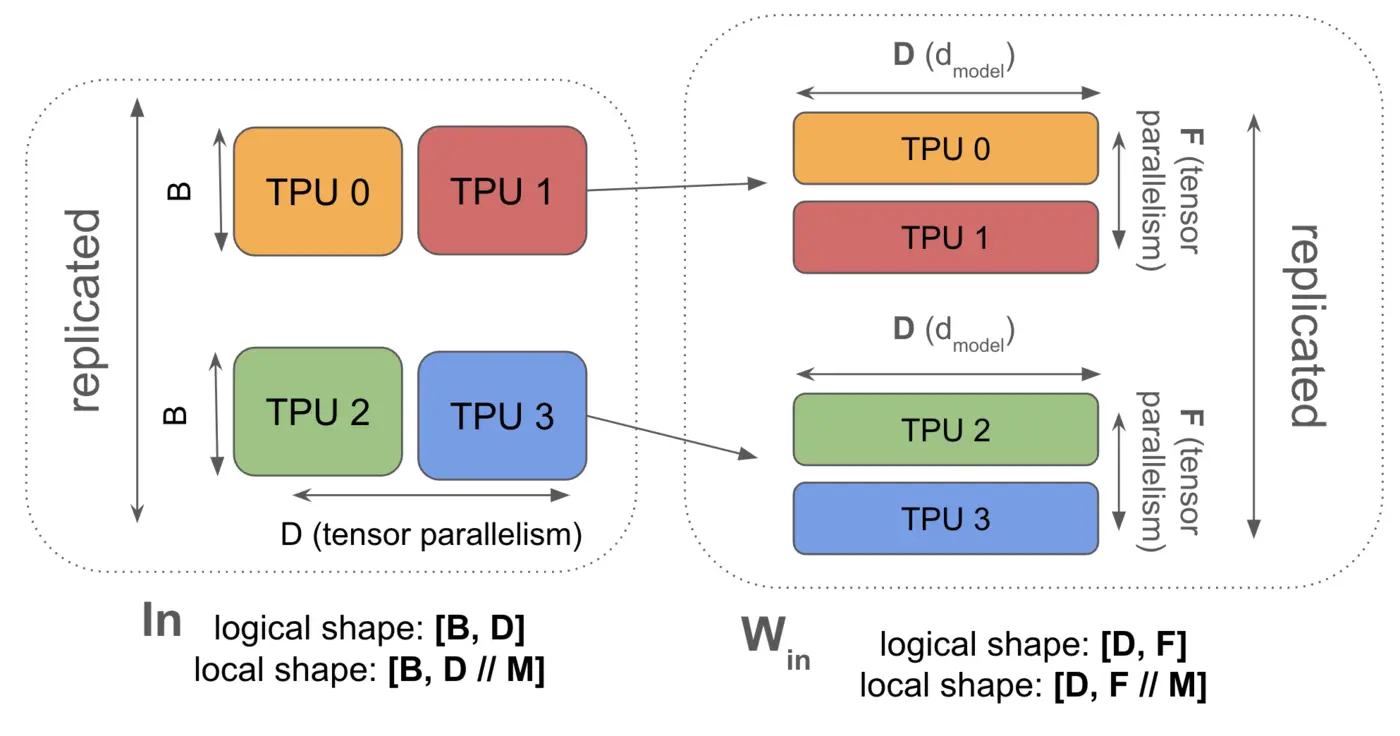
As noted, In[B, DY] *D Win[D, FY] *F Wout[FY, D] -> Out[B, DY] means we have to gather our activations before the first matmul. This is cheaper than ZeRO sharding when the activations are smaller than the weights. This is typically true only with some amount of ZeRO sharding added (which reduces the size of the gather). This is one of the reasons we tend to mix ZeRO sharding and tensor parallelism.
Here’s the algorithm for tensor parallelism!
Tensor Parallelism:
Forward pass: need to compute Loss[B]
- In[B, D] = AllGather(In[B, DY]) (on critical path)
- Tmp[B, FY] = In[B, D] *D Win[D, FY] (not sharded along contracting, so no comms)
- Out[B, D] {UY} = Tmp[B, FY] *F Wout[FY, D]
- Out[B, DY] = ReduceScatter(Out[B, D] {UY}) (on critical path)
- Loss[B] = …
Backward pass: need to compute dWout[FY, D], dWin[D, FY]
- dOut[B, DY] = …
- dOut[B, D] = AllGather(dOut[B, DY]) (on critical path)
- dWout[FY, D] = Tmp[B, FY] *B dOut[B, D]
- dTmp[B, FY] = dOut[B, D] *D Wout[FY, D] (can throw away dOut[B, D] here)
- In[B, D] = AllGather(In[B, DY]) (this can be skipped by sharing with (1) from the forward pass)
- dWin[D, FY] = In[B, D] *B dTmp[B, FY]
- dIn[B, D] {UY} = dTmp[B, FY] *F Win[D, FY] (needed for previous layers)
- dIn[B, DY] = ReduceScatter(dIn[B, D] {UY}) (on critical path)
One nice thing about tensor parallelism is that it interacts nicely with the two matrices in our Transformer forward pass. Naively, we would do an AllReduce after each of the two matrices. But here we first do In[B, DY] * Win[D, FY] -> Tmp[B, FY] and then Tmp[B, FY] * Wout[FY, D] -> Out[B, DY]. This means we AllGather In at the beginning, and ReduceScatter Out at the end, rather than doing an AllReduce.
How costly is this? Let’s only model the forward pass - the backwards pass is just the transpose of each operation here. In 1D tensor parallelism we AllGather the activations before the first matmul, and ReduceScatter them after the second, sending two bytes at a time (bf16). Let’s figure out when we’re bottlenecked by communication.
\[\begin{align} T_\text{math} & = \frac{4 \cdot B \cdot D \cdot F}{Y \cdot C} \\ T_\text{comms} & = \frac{2 \cdot 2 \cdot (B \cdot D)}{W_\text{ici}}\\ \textnormal{T} & \approx \max \left(\frac{4 \cdot B \cdot D \cdot F}{Y \cdot C}, \frac{2 \cdot 2 \cdot (B \cdot D)}{W_\text{ici}}\right) \end{align}\]Noting that we want compute cost to be greater than comms cost, we get:
\[\begin{align} \frac{4 \cdot B \cdot D \cdot F}{Y \cdot C} > \frac{2 \cdot 2 \cdot (B \cdot D)}{W_\text{ici}} \end{align}\] \[\begin{align} \frac{F}{Y \cdot C} > \frac{1}{W_\text{ici}} \end{align}\] \[\begin{align} F > Y \cdot \frac{C}{W_\text{ici}} \end{align}\]Thus for instance, for TPUv5p, $C / W_{ici} = 2550$ in bf16, so we can only do tensor parallelism up to $Y < F / 2550$. When we have multiple ICI axes, our $T_\text{comms}$ is reduced by a factor of $M_Y$, so we get $Y < M_Y \cdot F / 2550$.
Takeaway: Tensor Parallelism becomes communication bound when $Y > M_Y \cdot F / 2550$. For most models this is between 8 and 16-way tensor parallelism.
Note that this doesn’t depend on the precision of the computation, since e.g. for int8, on TPUv5p, \(C_\text{int8} / W_{ici}\) is \(5100\) instead of \(2550\) but the comms volume is also halved, so the two factors of two cancel.
Let’s think about some examples:
-
On TPUv5p with LLaMA 3-70B with \(D = 8192,\) \(F \approx 30,000\), we can comfortably do 8-way tensor parallelism, but will be communication bound on 16 way tensor parallelism. The required F for 8-way model sharding is 20k.
-
For Gemma 7B, \(F \approx 50k\), so we become communication bound with 19-way tensor parallelism. That means we could likely do 16-way and still see good performance.
Combining FSDP and Tensor Parallelism
Syntax: \(\text{In}[B_X, D_Y] \cdot_D W_\text{in}[D_X, F_Y] \cdot_F W_\text{out}[F_Y, D_X] \rightarrow \text{Out}[B_X, D_Y]\)
The nice thing about FSDP and tensor parallelism is that they can be combined. By sharding Win and Wout along both axes we both save memory and compute. Because we shard B along X, we reduce the size of the model-parallel AllGathers, and because we shard F along Y, we reduce the communication overhead of FSDP. This means a combination of the two can get us to an even lower effective batch size than we saw above.

Here’s the full algorithm for mixed FSDP + tensor parallelism. While we have a lot of communication, all our AllGathers and ReduceScatters are smaller because we have batch-sharded our activations and tensor sharded our weights much more!
Forward pass: need to compute Loss[B]
- In[BX, D] = AllGatherY(In[BX, DY]) (on critical path)
- Win[D, FY] = AllGatherX(Win[DX, FY]) (can be done ahead of time)
- Tmp[BX, FY] = In[BX, D] *D Win[D, FY]
- Wout[FY, D] = AllGatherX(Wout[FY, DX]) (can be done ahead of time)
- Out[BX, D] {UY} = Tmp[BX, FY] *F Wout[FY, D]
- Out[BX, DY] = ReduceScatterY(Out[BX, D] {UY}) (on critical path)
- Loss[BX] = …
Backward pass: need to compute dWout[FY, DX], dWin[DX, FY]
- dOut[BX, DY] = …
- dOut[BX, D] = AllGatherY(dOut[BX, DY]) (on critical path)
- dWout[FY, D] {UX} = Tmp[BX, FY] *B dOut[BX, D]
- dWout[FY, DX] = ReduceScatterX(dWout[FY, D] {UX})
- Wout[FY, D] = AllGatherX(Wout[FY, DX]) (can be done ahead of time)
- dTmp[BX, FY] = dOut[BX, D] *D Wout[FY, D] (can throw away dOut[B, D] here)
- In[BX, D] = AllGatherY(In[BX, DY]) (not on critical path + this can be shared with (2) from the previous layer)
- dWin[D, FY] {UX} = In[BX, D] *B dTmp[BX, FY]
- dWin[DX, FY] = ReduceScatterX(dWin[D, FY] {UX})
- Win[D, FY] = AllGatherX(Win[DX, FY]) (can be done ahead of time)
- dIn[BX, D] {UY} = dTmp[BX, FY] *F Win[D, FY] (needed for previous layers)
- dIn[BX, DY] = ReduceScatterY(dIn[BX, D] {UY}) (on critical path)
What’s the right combination of FSDP and TP? A simple but key maxim is that FSDP moves weights and tensor parallelism moves activations. That means as our batch size shrinks (especially as we do more data parallelism), tensor parallelism becomes cheaper because our activations per-shard are smaller.
- Tensor parallelism performs \(\mathbf{AllGather}_Y([B_X, D_Y])\) which shrinks as \(X\) grows.
- FSDP performs \(\mathbf{AllGather}_X([D_X, F_Y])\) which shrinks as \(Y\) grows.
Thus by combining both we can push our minimum batch size per replica down even more. We can calculate the optimal amount of FSDP and TP in the same way as above:
Let \(X\) be the number of chips dedicated to FSDP and \(Y\) be the number of chips dedicated to tensor parallelism. Let \(N\) be the total number of chips in our slice with \(N=XY\). Let \(M_X\) and \(M_Y\) be the number of mesh axes over which we do FSDP and TP respectively (these should roughly sum to 3). We’ll purely model the forward pass since it has the most communication per FLOP. Then adding up the comms in the algorithm above, we have
\[T_\text{FSDP comms}(B, X, Y) = \frac{2\cdot 2\cdot D \cdot F}{Y \cdot W_\text{ici} \cdot M_X}\] \[T_\text{TP comms}(B, X, Y) = \frac{2 \cdot 2 \cdot B \cdot D}{X \cdot W_\text{ici} \cdot M_Y}\]And likewise our total FLOPs time is
\[T_\text{math} = \frac{2\cdot 2 \cdot B \cdot D \cdot F}{N \cdot C}.\]To simplify the analysis, we make two assumptions: first, we allow $X$ and $Y$ to take on non-integer values (as long as they are positive and satisfy $XY=N$); second, we assume that we can fully overlap comms on the $X$ and $Y$ axis with each other. Under the second assumption, the total comms time is
\[T_\text{comms} = \max\left(T_\text{FSDP comms}, T_\text{TP comms}\right)\]Before we ask under what conditions we’ll be compute-bound, let’s find the optimal values for $X$ and $Y$ to minimize our total communication. Since our FLOPs is independent of $X$ and $Y$, the optimal settings are those that simply minimize comms. To do this, let’s write $T_\text{comms}$ above in terms of $X$ and $N$ (which is held fixed, as it’s the number of chips in our system) rather than $X$ and $Y$:
\[T_\text{comms} (X) = \frac{4D}{W_\text{ici}} \max\left(\frac{F \cdot X}{N \cdot M_X}, \frac{B}{X \cdot M_Y}\right)\]Because $T_\text{FSDP comms}$ is monotonically increasing in $X$, and $T_\text{TP comms}$ is monotonically decreasing in $X$, the maximum must be minimized when $T_\text{FSDP comms} = T_\text{TP comms}$, which occurs when
\[\begin{align*} \frac{FX_{opt}}{M_X} = \frac{BN}{X_{opt} M_Y} \rightarrow \\ X_{opt} = \sqrt{\frac{B}{F} \frac{M_X}{M_Y} N} \end{align*}\]This is super useful! This tells us, for a given $B$, $F$, and $N$, what amount of FSDP is optimal. Let’s get a sense of scale. Plugging in realistic values, namely $N = 64$ (corresponding to a 4x4x4 array of chips), $B=48,000$, $F=32768$, gives roughly $X\approx 13.9$. So we would choose $X$ to be 16 and $Y$ to be 4, close to our calculated optimum.
Takeaway: in general, during training, the optimal amount of FSDP is \(X_{opt} = \sqrt{\frac{B}{F} \frac{M_X}{M_Y} N}\).
Now let’s return to the question we’ve been asking of all our parallelism strategies: under what conditions will we be compute-bound? Since we can overlap FLOPs and comms, we are compute-bound when
\[\max\left(T_\text{FSDP comms}, T_\text{TP comms}\right) < T_\text{math}\]By letting $\alpha \equiv C / W_\text{ici}$, the ICI arithmetic intensity, we can simplify:
\[\max\left(\frac{F}{Y \cdot M_X}, \frac{B}{X \cdot M_Y}\right) < \frac{B \cdot F}{N \cdot \alpha}\]Since we calculated $X_{opt}$ to make the LHS maximum equal, we can just plug it into either side (noting that $Y_{opt} = N/X_{opt}$), i.e.
\[\frac{F}{N \cdot W_\text{ici} \cdot M_X} \sqrt{\frac{B}{F} \frac{M_X}{M_Y} N} < \frac{B \cdot F}{N \cdot C}\]Further simplifying, we find that
\[\sqrt{\frac{B\cdot F}{M_X \cdot M_Y \cdot N}} < \frac{B \cdot F}{N \cdot \alpha},\]where the left-hand-side is proportional to the communication time and the right-hand-side is proportional to the computation time. Note that while the computation time scales linearly with the batch size (as it does regardless of parallelism), the communication time scales as the square root of the batch size. The ratio of the computation to communication time thus also scales as the square root of the batch size:
\[\frac{T_\text{math}}{T_\text{comms}} = \frac{\sqrt{BF}\sqrt{M_X M_Y}}{\alpha \sqrt{N}}.\]To ensure that this ratio is greater than one so we are compute bound, we require
\[\frac{B}{N} > \frac{\alpha^2}{M_X M_Y F}\]To get approximate numbers, again plug in $F=32,768$, $\alpha=2550$, and $M_X M_Y=2$ (as it must be for a 3D mesh). This gives roughly $B/N > 99$. This roughly wins us a factor of eight compared to the purely data parallel (or FSDP) case, where assuming a 3D mesh we calculate that $B/N$ must exceed about $850$ to be compute bound.
Takeaway: combining tensor parallelism with FSDP allows us to drop to a $B/N$ of \(2550^2 / 2F\). This lets us handle a batch of as little as 100 per chip, which is roughly a factor of eight smaller than we could achieve with just FSDP.
Below we plot the ratio of FLOPs to comms time for mixed FSDP + TP, comparing it both to only tensor parallelism (TP) and only data parallelism (FSDP), on a representative 4x4x4 chip array. While pure FSDP parallelism dominates for very large batch sizes, in the regime where batch size over number of chips is between roughly 100 and 850, a mixed FSDP + TP strategy is required in order to be compute-bound.

Here’s another example of TPU v5p 16x16x16 showing the FLOPs and comms time as a function of batch size for different sharding schemes.

The black curve is the amount of time spent on model FLOPs, meaning any batch size where this is lower than all comms costs is strictly comms bound. You’ll notice the black curve intersects the green curve at about 4e5, as predicted.
Here’s an interactive animation to play with this, showing the total compute time and communication time for different batch sizes:
You’ll notice this generally agrees with the above (minimum around FSDP=256, TP=16), plus or minus some wiggle factor for some slight differences in the number of axes for each.
Pipelining
You’ll probably notice we’ve avoided talking about pipelining at all in the previous sections. Pipelining is a dominant strategy for GPU parallelism that is somewhat less essential on TPUs. Briefly, pipelined training involves splitting the layers of a model across multiple devices and passing the activations between pipeline stages during the forward and backward pass. The algorithm is something like:
- Initialize your data on TPU 0 with your weights sharded across the layer dimension ($W_\text{in}[L_Z, D_X, F_Y]$ for pipelining with FSDP and tensor parallelism).
- Perform the first layer on TPU 0, then copy the resulting activations to TPU 1, and repeat until you get to the last TPU.
- Compute the loss function and its derivative $\partial L / \partial x_L$.
- For the last pipeline stage, compute the derivatives $\partial L / \partial W_L$ and $\partial L / \partial x_{L-1}$, then copy $\partial L / \partial x_{L-1}$ to the previous pipeline stage and repeat until you reach TPU 0.
Here is some (working) Python pseudo-code
This pseudocode should run on a Cloud TPU VM. While it’s not very efficient or realistic, it gives you a sense how data is being propagated across devices.
batch_size = 32
d_model = 128
d_ff = 4 * d_model

num_layers = len(jax.devices())

key = jax.random.PRNGKey(0)

# Pretend each layer is just a single matmul.
x = jax.random.normal(key, (batch_size, d_model))
weights = jax.random.normal(key, (num_layers, d_model, d_model))

def layer_fn(x, weight):
  return x @ weight

# Assume we have num_layers == num_pipeline_stages
intermediates = [x]
for i in range(num_layers):
  x = layer_fn(x, weights[i])
  intermediates.append(x)

  if i != num_layers - 1:
    x = jax.device_put(x, jax.devices()[i+1])

def loss_fn(batch):
  return jnp.mean(batch ** 2)  # make up some fake loss function

loss, dx = jax.value_and_grad(loss_fn)(x)

for i in range(num_layers - 1, -1, -1):
  _, f_vjp = jax.vjp(layer_fn, intermediates[i], weights[i])
  dx, dw = f_vjp(dx)  # compute the jvp dx @ J(L)(x[i], W[i])
  weights[i] = weights[i] - 0.01 * dw  # update our weights

  if i != 0:
    dx = jax.device_put(dx, jax.devices()[i-1])
Why is this a good idea? Pipelining is great for many reasons: it has a low communication cost between pipeline stages, meaning you can train very large models even with low bandwidth interconnects. This is often very useful on GPUs since they are not densely connected by ICI in the way TPUs are.
Why is this difficult/annoying? You might have noticed in the pseudocode above that TPU 0 is almost always idle! It’s only doing work on the very first and last step of the pipeline. The period of idleness is called a pipeline bubble and is very annoying to deal with. Typically we try to mitigate this first with microbatching, which sends multiple small batches through the pipeline, keeping TPU 0 utilized for at least a larger fraction of the total step time.
A second approach is to carefully overlap the forward matmul $W_i @ x_i$, the backward $dx$ matmul $W_i @ \partial L / \partial x_{i+1}$, and the $dW$ matmul $\partial L / \partial x_{i+1} @ x_i$. Since each of these requires some FLOPs, we can overlap them to fully hide the bubble. Here’s a plot from the recent DeepSeek v3 paper

Because it is less critical for TPUs (which have larger interconnected pods), we won’t delve into this as deeply, but it’s a good exercise to understand the key pipelining bottlenecks.
Scaling Across Pods
The largest possible TPU slice is a TPU v5p SuperPod with 8960 chips (and 2240 hosts). When we want to scale beyond this size, we need to cross the Data-Center Networking (DCN) boundary. Each TPU host comes equipped with one or several NICs (Network Interface Cards) that connect the host to other TPU v5p pods over Ethernet. As noted in the TPU Section, each host has about 200Gbps (25GB/s) of full-duplex DCN bandwidth, which is about 6.25GB/s full-duplex (egress) bandwidth per TPU.
Typically, when scaling beyond a single pod, we do some form of model parallelism or FSDP within the ICI domain, and then pure data parallelism across multiple pods. Let $N$ be the number of TPUs we want to scale to and $M$ be the number of TPUs per ICI-connected slice. To do an AllReduce over DCN, we can do a ring-reduction over the set of pods, giving us (in the backward pass):
\[T_\text{math} = \frac{2 \cdot 2 \cdot 2 \cdot BDF}{N \cdot C}\] \[T_\text{comms} = \frac{2 \cdot 2 \cdot 2 \cdot DF}{M \cdot W_\text{dcn}}\]The comms bandwidth scales with $M$, since unlike ICI the total bandwidth grows as we grow our ICI domain and acquire more NICs. Simplifying, we find that $T_\text{math} > T_\text{comms}$ when
\[\frac{B}{\text{slice}} > \frac{C}{W_\text{dcn}}\]For TPU v5p, the $\frac{C}{W_\text{dcn}}$ is about 4.59e14 / 6.25e9 = 73,440. This tells us that to efficiently scale over DCN, there is a minimum batch size per ICI domain needed to egress each node.
How much of a problem is this? To take a specific example, say we want to train LLaMA-3 70B on TPU v5p with a BS of 2M tokens. LLaMA-3 70B has $F\approx 30,000$. From the above sections, we know the following:
- We can do Tensor Parallelism up to $Y = M_Y \cdot F / 2550 \approx 11 \cdot M_Y$.
- We can do FSDP so long as $B / N > 2550 / M_X$. That means if we want to train with BS=2M and 3 axes of data parallelism, we’d at most be able to use $\approx 2400$ chips, roughly a quarter of a TPU v5p pod.
- When we combine FSDP + Tensor Parallelism, become comms-bound when we have $B / N < 2550^2 / (2 \cdot 30000) = 108$, so this lets us scale to roughly 18k chips! However, the maximum size of a TPU v5p pod is 8k chips, so beyond that we have to use DCN.
The TLDR is that we have a nice recipe for training with BS=1M, using roughly X (FSDP) = 1024 and Y (TP) = 8, but with BS=2M we need to use DCN. As noted above, we have a DCN arithmetic intensity of $\text{73,440}$, so we just need to make sure our batch size per ICI domain is greater than this. This is trivial for us, since with 2 pods we’d have a per-pod BS of 1M, and a per TPU batch size of 111, which is great (maybe cutting it a bit close, but theoretically sound).
Takeaway: Scaling across multiple TPU pods is fairly straightforward using pure data parallelism so long as our per-pod batch size is at least 73k tokens.
Takeaways from LLM Training on TPUs
-
Increasing parallelism or reducing batch size both tend to make us more communication-bound because they reduce the amount of compute performed per chip.
-
Up to a reasonable context length (~32k) we can get away with modeling a Transformer as a stack of MLP blocks and define each of several parallelism schemes by how they shard the two/three main matmuls per layer.
-
During training there are 4 main parallelism schemes we consider, each of which has its own bandwidth and compute requirements (data parallelism, FSDP, tensor parallelism, and mixed FSDP + tensor parallelism).
| Strategy | Description |
|---|---|
| Data Parallelism | Activations are batch sharded, everything else is fully-replicated, we all-reduce gradients during the backward pass. |
| FSDP | Activations, weights, and optimizer are batch sharded, weights are gathered just before use, gradients are reduce-scattered. |
| Tensor Parallelism (aka Megatron, Model) | Activations are sharded along \(d_\text{model}\), weights are sharded along \(d_{ff}\), activations are gathered before Win, the result reduce-scattered after Wout. |
| Mixed FSDP + Tensor Parallelism | Both of the above, where FSDP gathers the model sharded weights. |
And here are the “formulas” for each method:
\[\small \begin{array}{cc} \text{Strategy} & \text{Formula}\\ \hline \text{DP} & \text{In}[B_X, D] \cdot_D W_\text{in}[D, F] \cdot_F W_\text{out}[F, D] \rightarrow \text{Out}[B_X, D] \\ \text{FSDP} & \text{In}[B_X, D] \cdot_D W_\text{in}[D_X, F] \cdot_F W_\text{out}[F, D_X] \rightarrow \text{Out}[B_X, D] \\ \text{TP} & \text{In}[B, D_Y] \cdot_D W_\text{in}[D, F_Y] \cdot_F W_\text{out}[F_Y, D] \rightarrow \text{Out}[B, D_Y] \\ \text{TP + FSDP} & \text{In}[B_X, D_Y] \cdot_D W_\text{in}[D_X, F_Y] \cdot_F W_\text{out}[F_Y, D_X] \rightarrow \text{Out}[B_X, D_Y] \\ \hline \end{array}\]- Each of these strategies has a limit at which it becomes network/communication bound, based on their per-device compute and comms. Here’s compute and comms per-layer, assuming \(X\) is FSDP and \(Y\) is tensor parallelism.
-
Pure data parallelism is rarely useful because the model and its optimizer state use bytes = 10x parameter count. This means we can rarely fit more than a few billion parameters in memory.
-
Data parallelism and FSDP become comms bound when the \(\text{batch size per shard} < C / W\), the arithmetic intensity of the network. For ICI this is 2,550 and for DCN this is about 71,000. This can be increased with more parallel axes.
-
Tensor parallelism becomes comms bound when \(\lvert Y\rvert > F / 2550\). This is around 8-16 way for most models. This is independent of the batch size.
-
Mixed FSDP + tensor parallelism allows us to drop the batch size to as low as \(2550^2 / 2F \approx 100\). This is remarkably low.
-
Data parallelism across pods requires a minimum batch size per pod of roughly 71,000 before becoming DCN-bound.
-
Basically, if your batch sizes are big or your model is small, things are simple. You can either do data parallelism or FSDP + data parallelism across DCN. The middle section is where things get interesting.
Some Problems to Work
Let’s use LLaMA-2 13B as a basic model for this section. Here are the model details:
| hyperparam | value |
|---|---|
| L | 40 |
| D | 5,120 |
| F | 13824 |
| N | 40 |
| K | 40 |
| H | 128 |
| V | 32,000 |
LLaMA-2 has separate embedding and output matrices and a gated MLP block.
Question 1: How many parameters does LLaMA-2 13B have (I know that’s silly but do the math)? Note that, as in Transformer Math, LLaMA-3 has 3 big FFW matrices, two up-projection and one down-projection. We ignored the two “gating” einsum matrices in this section, but they behave the same as Win in this section.
Click here for the answer.
- FFW parameters: \(3LDF\) =
8.5e9 - Attention parameters: \(4DNHL\) =
4.2e9 - Vocabulary parameters: \(2VD\) =
0.33e9 - Total:
8.5e9 + 4.2e9 + 0.33e9 = 13.0e9, as expected!
Question 2: Let’s assume we’re training with BS=16M tokens and using Adam. Ignoring parallelism for a moment, how much total memory is used by the model’s parameters, optimizer state, and activations? Assume we store the parameters in bf16 and the optimizer state in fp32 and checkpoint activations three times per layer (after the three big matmuls).
Click here for the answer.
The total memory used for the parameters (bf16) and the two optimizer states (fp32, the first and second moment accumulators) is (2 + 4 + 4) * 13e9 ~ 130GB. The activations after the first two matmuls are shaped $BF$ and after the last one $BD$ (per the Transformer diagram above), so the total memory for bf16 is $2 \cdot L \cdot (BD + 2 * BF) = 2LB \cdot (D + 2F)$ or 2 * 40 * 16e6 * 5,120 * (1 + 2 * 2.7) ~ 4.2e13 = 42TB, since B=16e6. All other activations are more or less negligible.
Question 3: Assume we want to train with 32k sequence length and a total batch size of 3M tokens on a TPUv5p 16x16x16 slice. Assume we want to use bfloat16 weights and a float32 optimizer, as above.
- Can we use pure data parallelism? Why or why not?
- Can we use pure FSDP? Why or why not? With pure FSDP, how much memory will be used per device (assume we do gradient checkpointing only after the 3 big FFW matrices).
- Can we use mixed FSDP + tensor parallelism? Why or why not? If so, what should $X$ and $Y$ be? How much memory will be stored per device? Using only roofline FLOPs estimates and ignoring attention, how long will each training step take at 40% MFU?
Click here for the answer.
First, let’s write down some numbers. With 32k sequence length and a 3M batch size, we have a sequence batch size of 96. On a TPU v5p 16x16x16 slice, we have 393TB of HBM.
-
We can’t use pure data parallelism, because it replicates the parameters and optimizer states on each chip, which are already around 130GB (from Q2) which is more HBM than we have per-chip (96GB).
-
Let’s start by looking purely at memory. Replacing BS=16M with 3M in Q2, we get
~7.86e12total checkpoint activations, and with the 1.3e11 optimizer state this brings us to almost exactly 8e12 = 8TB. The TPUv5p slice has393TBof HBM in total, so we are safely under the HBM limit. Next let’s look at whether we’ll be comms or compute-bound. With 4096 chips and 3 axes of parallelism, we can do a minimum batch size of850 * 4096 = 3.48Mtokens. That’s slightly above our 3M batch size. So we’re actually comms-bound, which is sad. So the general answer is no, we cannot do FSDP alone. -
Now we know our primary concern is being comms-bound, so let’s plug in some numbers. First of all, we know from above that our per-chip batch size with mixed FSDP + tensor parallelism needs to be above $2550^2 / 2F = 235$ here. That means we can in theory do this! Let’s figure out how much of each.
We have the rule $X_{opt} = \sqrt{(B / F) \cdot (M_X / M_Y) \cdot N}$, so here we have sqrt(3e6 * 2 * 4096 / 13824) = 1333, meaning we’ll do roughly 1024 way DP and 4 way TP. Per TPU memory will be as in (2), and step time will just be 6 * 3e6 * 13e9 / (4096 * 4.6e14 * 0.4) = 300ms.
That’s it for Part 5! For Part 6, which applies this content to real LLaMA models, click here!
Appendix
Appendix A: Deriving the backward pass comms
Above, we simplified the Transformer layer forward pass as Out[B, D] = In[B, D] *D Win[D, F] *F Wout[F, D]. How do we derive the comms necessary for the backwards pass?
This follows fairly naturally from the rule in the previous section for a single matmul Y = X * A:
\[\frac{dL}{dA} = \frac{dL}{dY}\frac{dY}{dA} = X^T \left(\frac{dL}{dY}\right)\] \[\frac{dL}{dX} = \frac{dL}{dY}\frac{dY}{dX} = \left(\frac{dL}{dY}\right) A^T\]Using this, we get the following formulas (letting Tmp[B, F] stand for In[B, D] * Win[D, F]):
- dWout[F, D] = Tmp[B, F] *B dOut[B, D]
- dTmp[B, F] = dOut[B, D] *D Wout[F, D]
- dWin[D, F] = In[B, D] *B dTmp[B, F]
- dIn[B, D] = dTmp[B, F] *F Win[D, F]
Note that these formulas are mathematical statements, with no mention of sharding. The job of the backwards pass is to compute these four quantities. So to figure out the comms necessary, we just take the shardings of all the quantities which are to be matmulled in the four equations above (Tmp, dOut, Wout, Win), which are specified by our parallelization scheme, and use the rules of sharded matmuls to figure out what comms we have to do. Note that dOut is sharded in the same way as Out.