All About Rooflines
Part 1 of How To Scale Your Model (Part 0: Introduction | Part 2: TPUs)
When we run algorithms on hardware, we're bounded by three things: how fast our computer can do math (OPs/second), the bandwidth available for moving data around (bytes/second), and the total memory available to store data (bytes). These "roofline" constraints let us upper and lower bound the time of a given computation.
Where Does the Time Go?
Let’s start with an extremely simple question: why does an algorithm take 50ms instead of 50s or 5ms? What is actually happening within the model that takes substantial time and how long should we expect it to take?
Computation: A deep learning model is effectively a bunch of matrix multiplications, each composed of floating-point multiplication and addition ‘operations’ (FLOPs). Our accelerator speed determines how long these take to compute:
\[\begin{equation} T_\text{math} = \frac{\text{Computation FLOPs}}{\text{Accelerator FLOPs/s}} \end{equation}\]For instance, an NVIDIA H100 can perform about 9.89e14 bfloat161e12 / 9.89e14 = 1.01ms and 1e12 / 9.1e14 = 1.1ms on a TPU v6e.
Communication within a chip: Within an accelerator, tensors need to be transferred between accelerator memory (HBM) and the compute cores. You’ll see the bandwidth of this link referred to as “HBM bandwidth”.
Communication between chips: When we distribute a model across multiple accelerators, tensors frequently need to be transferred between them. There are often a few options for this on our hardware (ICI, DCN, and PCIe), each with different bandwidths.
Whether the communication is within a chip or between chips, we measure this in bytes/s and estimate the total communication time with:
\[\begin{equation} T_\text{comms} = \frac{\text{Communication Bytes}}{\text{Network/Memory Bandwidth Bytes/s}} \end{equation}\]Typically (but not always), computation within a single chip can be overlapped with communication within a chip and between chips. This means we can lower-bound training and inference time by using the maximum of computation and communication time. We can also upper-bound with their sum. In practice, we optimize against the maximum as the algebra is simpler and we can usually come close to this bound by overlapping our communication and computation. If we optimize with the maximum in mind then the lower and upper bounds differ by at most a factor of 2 since $T_\text{math} + T_\text{comms} \leq 2 * \max(T_\text{math}, T_\text{comms})$. We then increase accuracy beyond this by modeling ‘overlap regions’ and overheads, which can be informed by profiling your specific model and target system.
\[\begin{equation} T_\text{lower}=\max(T_\text{math}, T_\text{comms}) \end{equation}\] \[\begin{equation} T_\text{upper} = T_\text{math} + T_\text{comms} \end{equation}\]If we assume we can perfectly overlap communication and computation, when $T_\text{math} > T_\text{comms}$, we see full utilization from our hardware. We call this being “compute-bound”. When $T_\text{comms} > T_\text{math}$, we tend to be “communication-bound”
Definition: the arithmetic intensity of an algorithm is given by the ratio of the total FLOPs it performs to the number of bytes it needs to communicate — either within a chip or between chips.
\[\begin{equation} \text{Arithmetic Intensity} = \frac{\text{Computation FLOPs}}{\text{Communication Bytes}} \end{equation}\]Arithmetic intensity measures the “FLOPs per byte” of a given operation. To a first order, when our arithmetic intensity is high, $T_\text{math}$ is large compared to $T_\text{comms}$ and we typically use most of the available FLOPs. When the opposite is true, we spend more time on comms and waste FLOPs. The point where this crossover happens is the “peak arithmetic intensity” of our hardware, the ratio of peak accelerator FLOPs/s to accelerator bandwidth.
\[\begin{align*} T_\text{math} > T_\text{comms} \Leftrightarrow \frac{\text{Computation FLOPs}} {\text{Accelerator FLOPs/s}} > \frac{\text{Communication Bytes}}{\text{Bandwidth Bytes/s}} & \\[0.5em] \Leftrightarrow \frac{\text{Computation FLOPs}}{\text{Communication Bytes}} > \frac{\text{Accelerator FLOPs/s}}{\text{Bandwidth Bytes/s}} & \\[0.5em] \Leftrightarrow \text{Intensity}(\text{Computation}) > \text{Intensity}(\text{Accelerator}) & \\ \end{align*}\]The quantity $\text{Intensity}(\text{Accelerator})$ is the arithmetic intensity at which our accelerator achieves its peak FLOPs/s. For the TPU v5e MXU, this is about 240 FLOPs/byte, since the TPU can perform 1.97e14 FLOPs/s and load 8.2e11 bytes/s from HBM.
Example (dot product): to compute the dot product of two vectors in bfloat16 precision, x • y: bf16[N], bf16[N] → bf16[1], we need to load $x$ and $y$ from memory, each of which has $2 * N = 2N$ bytes, perform $N$ multiplications and $N-1$ additions, and write $2$ bytes back into HBM \(\begin{equation} \text{Intensity}(\text{dot product}) = \frac{\text{Total FLOPs}}{\text{Total Bytes}} = \frac{N + N - 1}{2N + 2N + 2} = \frac{2N - 1}{4N + 2} \rightarrow \frac{1}{2} \end{equation}\)
as $N\rightarrow\infty$. So the dot product has an arithmetic intensity of $\frac{1}{2}$ or, put another way, the dot product does 0.5 floating point operations per byte loaded. This means our arithmetic intensity is lower than that of our hardware and we will be communication-bound.
Visualizing rooflines
We can visualize the tradeoff between memory and compute using a roofline plot, which plots the peak achievable FLOPs/s (throughput) of an algorithm on our hardware (the y-axis) against the arithmetic intensity of that algorithm (the x-axis). Here’s an example log-log plot:
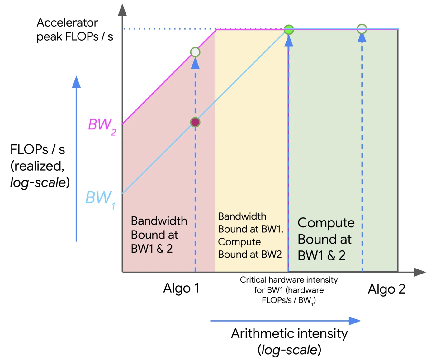
Above, as the intensity increases (moving left to right), we initially see a linear increase in the performance of our algorithm (in FLOPs/s) until we hit the critical arithmetic intensity of the hardware, 240 in the case of the TPU v5e. Any algorithm with a lower intensity will be bandwidth (BW) bound and limited by the peak memory bandwidth (shown in red). Any algorithm to the right will fully utilize our FLOPs (shown in green). Here, Algo 1 is comms-bound and uses only a fraction of the total hardware FLOPs/s. Algo 2 is compute-bound. We can generally improve the performance of an algorithm either by increasing its arithmetic intensity or by increasing the memory bandwidth available (moving from BW1 to BW2).
Matrix multiplication
Let’s look at our soon-to-be favorite algorithm: matrix multiplication (aka matmul). We write $X * Y \rightarrow Z$ where $X$ has shape $\text{bf16}[B, D]$, $Y$ has shape $\text{bf16}[D, F]$, and $Z$ has shape $\text{bf16}[B, F]$. To do the matmul we need to load $2DF + 2BD$ bytes, perform $2BDF$ FLOPs, and write $2BF$ bytes back.
We can get a nice simplification if we assume our “batch size” $B$ is small relative to $D$ and $F$. Then we get
\[\begin{equation} \frac{BDF}{BD + DF + BF} \approx \frac{BDF}{DF} = B \end{equation}\] \[\begin{equation} \text{Intensity}(\text{matmul}) > \text{Intensity}(\text{TPU}) \implies B > \frac{1.97e14}{8.20e11} = 240 \end{equation}\]This is a reasonable assumption for Transformer matmuls since we typically have a local (per-replica) batch size $B < 1024$ tokens (not sequences) but $D$ and $F > 8000$. Thus we generally become compute-bound when our per-replica
Takeaway: for a bfloat16 matmul to be compute-bound on most TPUs, we need our per-replica token batch size to be greater than 240.
This comes with a few notable caveats we’ll explore in the problems below, particularly with respect to quantization (e.g., if we quantize our activations but still do full-precision FLOPs), but it’s a good rule to remember. For GPUs, this number is slightly higher (closer to 300), but the same conclusion generally holds. When we decompose a big matmul into smaller matmuls, the tile sizes also matter.
Network communication rooflines
All the rooflines we’ve discussed so far have been memory-bandwidth rooflines, all within a single chip. This shouldn’t be taken as a rule. In fact, most of the rooflines we’ll care about in this book involve communication between chips: usually matrix multiplications that involve matrices sharded across multiple TPUs.
To pick a somewhat contrived example, say we want to multiply two big matrices $X\sim \text{bf16}[B, D]$ and $Y \sim \text{bf16}[D, F]$ which are split evenly across 2 TPUs/GPUs (along the $D$ dimension). To do this multiplication (as we’ll see in Section 3), we can multiply half of each matrix on each TPU (Z0 = X[:, :D // 2] @ Y[:D // 2, :] on TPU 0 and Z1 = X[:, D // 2:] @ Y[D // 2:, :] on TPU 1) and then copy the resulting “partial sums” to the other TPU and add them together. Say we can copy 4.5e10 bytes/s in each direction and perform 1.97e14 FLOPs/s on each chip. What are $T_\text{math}$ and $T_\text{comms}$?
$T_\text{math}$ is clearly half of what it was before, since each TPU is doing half the work, i.e.
Now what about $T_\text{comms}$? This now refers to the communication time between chips! This is just the total bytes sent divided by the network bandwidth, i.e.
\[T_\text{comms} = \frac{2BF}{\text{Network Bandwidth}} = \frac{2BF}{4.5e10}\]Therefore we become compute-bound (now with respect to the inter-chip network) when \(\text{Intensity}(\text{matmul (2-chips)}) > \text{Intensity}(\text{TPU w.r.t. inter-chip network})\) or equivalently when $\frac{BDF}{2BF} = \frac{D}{2} > \frac{1.97e14}{4.5e10} = 4377$ or $D > 8755$. Note that, unlike before, the critical threshold now depends on $D$ and not $B$! Try to think why that is. This is just one such example, but we highlight that this kind of roofline is critical to knowing when we can parallelize an operation across multiple TPUs.
A Few Problems to Work
Question 1 [int8 matmul]: Say we want to do the matmul $X[B, D] \cdot_D Y[D, F] \rightarrow Z[B, F]$
- How many bytes need to be loaded from memory? How many need to be written back to memory?
- How many total OPs are performed?
- What is the arithmetic intensity?
- What is a roofline estimate for $T_\text{math}$ and $T_\text{comms}$? What are reasonable upper and lower bounds for the runtime of the whole operation?
Assume our HBM bandwidth is 8.2e11 bytes/s and our int8 peak OPs/s is 3.94e14 (about 2x bfloat16).
Click here for the answer.
- Because we’re storing our parameters in int8, we have 1 byte per parameter, so we have \(BD + DF\) bytes loaded from HBM and \(BF\) written back.
- This is the same as in bfloat16, but in theory int8 OPs/s should be faster. So this is still $2BDF$ OPs.
- Arithmetic intensity is \(2BDF / (BD + DF + BF)\). If we make the same assumption as above about \(B \ll D\) and \(B \ll F\), we get an arithmetic intensity of \(2B\), meaning our rule becomes $B > \text{HBM int8 arithmetic intensity} / 2$. Using the numbers given, this int8 intensity is
3.94e14 / 8.2e11 = 480, so the rule is $B > 480 / 2 = 240$. Note that this is basically unchanged! - \(T_\text{math} = 2BDF / 3.94e14\) and \(T_\text{comms} = (BD + DF + BF) / 8.2e11\), so a reasonable lower bound is \(\max(T_\text{math}, T_\text{comms})\) and an upper bound is \(T_\text{math} + T_\text{comms}\).
Question 2 [int8 + bf16 matmul]: In practice we often do different weight vs. activation quantization, so we might store our weights in very low precision but keep activations (and compute) in a higher precision. Say we want to quantize our weights in int8 but keep activations (and compute) in bfloat16. At what batch size do we become compute bound? Assume 1.97e14 bfloat16 FLOPs/s.
Hint: this means specifically bf16[B, D] * int8[D, F] -> bf16[B, F] where $B$ is the “batch size”.
Click here for the answer.
Again assuming B is small, we have 2BDF bfloat16 FLOPs but only DF weights (instead of 2DF in bfloat16). This means we become compute-bound when \(2B > 240\) or \(B > 120\). This is a lot lower, meaning if we can do int8 weight quantization (which is fairly easy to do) but still do bfloat16 FLOPs, we get a meaningful win in efficiency (although int8 OPs would be better).
Question 3: Taking the setup from Question 2, make a roofline plot of peak FLOPs/s vs. $B$ for $F = D = 4096$ and $F = D = 1024$. Use the exact number of bytes loaded, not an approximation.
Click here for the answer.
Here is the plot in question:

Note that both models eventually achieve the peak hardware FLOPs/s, but the larger D/F achieve it sooner. D=F=1024 almost doubles the critical batch size. The code to generate this figure is here:
import matplotlib.pyplot as plt
import numpy as np

bs = np.arange(1, 512)

def roofline(B, D, F):
  total_flops = 2*B*D*F
  flops_time = total_flops / 1.97e14
  comms_time = (2*B*D + D*F + 2*B*F) / 8.2e11
  total_time = np.maximum(flops_time, comms_time)
  return total_flops / total_time

roofline_big = roofline(bs, 4096, 4096)
roofline_small = roofline(bs, 1024, 1024)

plt.figure(figsize=(8, 4))
plt.plot(bs, roofline_big, label='F=D=4096')
plt.plot(bs, roofline_small, label='F=D=1024')
plt.legend()
plt.xlabel('batch size')
plt.ylabel('peak bfloat16 FLOPs/s on TPU v5e')
plt.grid()
Question 4: What if we wanted to perform $\text{int8}[B, D] \cdot_D \text{int8}[B, D, F] \rightarrow \text{int8}[B, F]$ where we imagine having a different matrix for each batch element. What is the arithmetic intensity of this operation?
Click here for the answer.
Let’s start by looking at the total FLOPs and comms.
- Total FLOPs: the FLOPs is basically the same, since we’re doing \(B\) independent \([D] \times [D, F]\) products, the same total work as a single \([B, D] \times [D, F]\) matmul (this is discussed more in Section 4). So this is just \(2BDF\).
- Total comms: we have a lot more comms here: \(BD + BDF + BF\).
- Therefore, our arithmetic intensity is now actually \(2BDF / (BD + BDF + BF)\). Since \(BDF\) dominates the denominator, this is roughly \(2\). So instead of it depending on the batch size, this is essentially constant. This is bad because it means we’ll basically always be comms bound no matter what.
Question 5 [Memory Rooflines for GPUs]: Using the spec sheet provided by NVIDIA for the H100 SXM, calculate the batch size at which a bfloat16 matrix multiplication will become compute-bound. Note that the Tensor Core FLOPs numbers are twice the true value since they’re only achievable with structured sparsity.
Click here for the answer.
From the spec sheet, we see that the reported bfloat16 FLOPs value is 1.979e15 FLOPs/s with an asterisk noting “with sparsity”. The true value is half this without sparsity, i.e. 9.89e14 FLOPs/s. The memory bandwidth is 3.35TB/s, or 3.35e12 bytes / second. Thus $B_\text{crit}$ is 9.89e14 / 3.35e12 = 295, rather similar to the TPU.