All About Transformer Inference
Part 7 of How To Scale Your Model (Part 6: Training LLaMA | Part 8: Serving LLaMA)
Performing inference on a Transformer can be very different from training. Partly this is because inference adds a new factor to consider: latency. In this section, we will go all the way from sampling a single new token from a model to efficiently scaling a large Transformer across many slices of accelerators as part of an inference engine.
The Basics of Transformer Inference
So you’ve trained a Transformer, and you want to use it to generate some new sequences. At the end of the day, benchmark scores going up and loss curves going down are only proxies for whether something interesting is going to happen once the rubber hits the road!
Sampling is conceptually simple. We put a sequence in and our favorite Transformer will spit out \(\log p(\text{next token}_i \vert \text{previous tokens})\), i.e. log-probabilities for all possible next tokens. We can sample from this distribution and obtain a new token. Append this token and repeat this process and we obtain a sequence of tokens which is a continuation of the prompt.
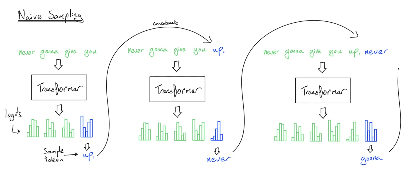
We have just described the naive implementation of Transformer sampling, and while it works, we never do it in practice because we are re-processing the entire sequence every time we generate a token. This algorithm is \(O(n^2)\) on the FFW and \(O(n^3)\) on the attention mechanism to generate \(n\) tokens!
How do we avoid this? Instead of doing the full forward pass every time, it turns out we can save some intermediate activations from each forward pass that let us avoid re-processing previous tokens. Specifically, since a given token only attends to previous tokens during dot-product attention, we can simply write each token’s key and value projections into a new data structure called a KV cache. Once we’ve saved these key/value projections for past tokens, future tokens can simply compute their \(q_i \cdot k_j\) products without performing any new FLOPs on the earlier tokens. Amazing!
With this in mind, inference has two key parts:
- Prefill: Given a long prompt, we process all the tokens in the prompt at the same time and save the resulting activations (specifically, the key-value projections) in a “KV cache”. We also save the logits for the last token.
- Generation: Given a KV cache and the previous logits, we incrementally sample one token from the logits, feed that token back into the Transformer, and produce a new set of logits for the next step. We also append the KV activations for that new token to the KV cache. We repeat this until we hit a special
<EOS>token or reach some maximum length limit.
Here’s a diagram of sampling with a KV cache:
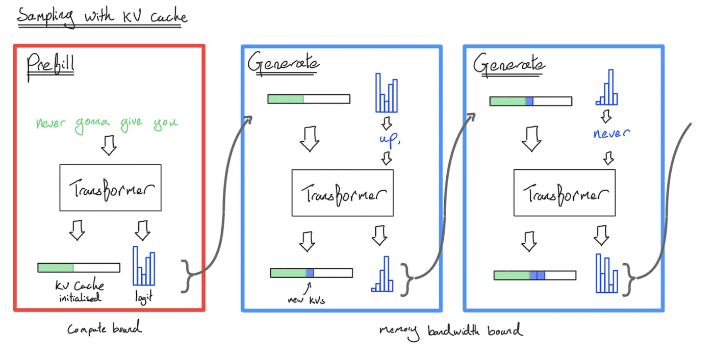
By sampling with a KV cache, we’ve reduced our time complexity to generate $n$ tokens to \(O(n)\) on the FFW and \(O(n^2)\) on the attention, since we never reprocess a previous token. However, many forward passes are still needed to generate a sequence — that’s what’s happening when you query Gemini or ChatGPT and the result streams back to you. Every token is (usually) a separate (but partially cached) Transformer call to a massive model.
We will soon see that prefill and generation are very different beasts — Transformer inference is two tasks in disguise! Compared to training, the KV cache is also a novel and significant source of complexity.
What do we actually want to optimize?
Before we proceed further, it’s worth highlighting one aspect of inference that’s totally new: latency. While during training we only care about throughput (total tokens processed per second per chip), during inference we have to worry about how fast we’re producing tokens (both the Time To First Token (TTFT) and the per-token latency). For example:
- Offline batch inference for evals and data generation only cares about bulk cost of inference and is blind to the latency of individual samples.
- Chat interfaces/streaming tasks need to run cheaply at scale while having low TTFT and generating tokens fast enough to exceed human reading speed.
- Edge inference (e.g.
llama.cppon your laptop) only needs to service one user at a time at the lowest possible latency, potentially with heavy hardware constraints.
Maximizing hardware utilization is still critical and helps with cost and TTFT, but unlike training, it does not necessarily translate to better experience for individual users in all contexts. Many optimizations at the accelerator, systems and model architectural level make tradeoffs between latency, throughput, context length and even model quality.
A more granular view of the Transformer
So far we’ve mostly treated a Transformer as a stack of feedforward blocks. While this is often reasonable from a FLOPs and memory standpoint, it’s not sufficient to properly model inference.
- A bunch of linear operations, including the MLP ($W_{in}$, $W_{out}$) and the attention QKV projections and output projections ($W_Q$, $W_K$, $W_V$, and $W_O$). These all involve reading parameters and a batch of activations from HBM, doing some FLOPs, and writing the result back to HBM.
- Dot-product attention. We need to read a batch of key-value projections and a batch of query activations from HBM, do a few inner products and some softmax operations, and write the attention result back to HBM.
- Everything else, including applying layer norms, activation functions, token sampling, updating KV caches, and positional embeddings. These do take some FLOPs, but are dominated by, or fused into, the above.
For the next couple of sections, we’re going to look at each of these in the context of prefill and generation and ask what is likely to bottleneck our performance. Within a single accelerator, are we compute-bound or memory-bound? We want to emphasize how different the answers will be for prefill versus generation.
Linear operations: what bottlenecks us?
All our linear operations are conceptually the same, whether they live in the MLP block or attention. Their arithmetic intensity depends on the batch size. We did this math in Section 1 but it’s worth repeating. Let’s look at a single matrix multiply of a $\text{bf16[B, D]}$ batch by a $\text{bf16[D, F]}$ matrix. This could be the big MLP block ($W_\text{in}$ or $W_\text{out}$) or one of the smaller attention projections ($W_Q$, $W_K$, $W_V$, $W_O$). To do this matmul, we need to load both of these arrays from HBM into the MXU, do the multiplication, then write the result back to HBM. As before, we have:
\[T_\text{math} = \frac{\text{Computation FLOPs}}{\text{Accelerator FLOPs/s}} = \frac{2BDF}{\text{Accelerator FLOPs/s}}\] \[T_\text{comms} = \frac{\text{Communication Bytes}}{\text{Bandwidth Bytes/s}} = \frac{2BD + 2FD + 2BF}{\text{Bandwidth Bytes/s}}\]A TPU or GPU can overlap these by loading as it does the compute, so to be compute-bound, we need \(T_\text{math} \geq T_\text{comms}\), or:
\[\frac{2BDF}{2BD + 2DF + 2BF} \geq \frac{\text{Accelerator FLOPs/s}}{\text{Bandwidth Bytes/s}} \underset{\text{TPU v5e}}{=} \frac{1.97E+14}{8.20E+11} = 240\]where the RHS is the arithmetic intensity of our hardware. Now let’s assume $D$ and $F$ are very large compared to $B$ (usually our batches are at most 500 and $D$ and $F > 10k$), we can simplify the denominator by using the fact that $\small{2BD + 2DF + 2BF \approx 2DF}$ which gives us
\[\begin{align*} \frac{2BDF}{2BD + 2DF + 2BF} \approx \frac{2BDF}{2DF} \geq \frac{\text{Accelerator FLOPs/s}}{\text{Bandwidth Bytes/s}} \\ \underset{\text{TPU v5e}}{=} \frac{1.97E+14}{8.20E+11} \implies B \geq 240 = B_{\text{crit}} \end{align*}\]If we quantize our weights or use lower precision FLOPs for the matrix multiplication, this critical batch size can change. For instance, if we quantize our weights to int8 or fp8, $B_\text{crit}$ decreases by 2x. If we do our FLOPs in int8 or fp8, $B_\text{crit}$ increases by 2x. Thus if we let $\beta = \text{bits per param} / \text{bits per activation}$ and $\alpha_\text{hbm} = C / W_\text{hbm}$, our critical batch size is actually $B_\text{crit} = \beta \alpha_\text{hbm}$.
Takeaway: Transformer matmuls are compute-bound iff the per-replica token batch size is greater than $B_\text{crit} = C / W_\text{hbm} \cdot (\text{bits per param} / \text{bits per activation}) = \beta \cdot \alpha_\text{hbm}$. For bf16 activations on TPU v5e, this is 240 tokens. For an H100, it is about 280 tokens.
During training, we’ll have a high intensity during all our matrix multiplications because we reuse the same weights over a very large batch. That high arithmetic intensity carries over to prefill, since user prompts are typically hundreds if not thousands of tokens long. As we saw before, the hardware arithmetic intensity of a TPUv5e is 240, so if a sequence longer than 240 tokens is fed into a dense model running on this hardware at bf16, we would expect to be compute-bound and all is well. Prompts shorter than this can technically be batched together to achieve higher utilization, but this is typically not necessary.
Takeaway: During prefill, all matrix multiplications are basically always compute-bound. Therefore, simply maximizing hardware utilization or MFU (Model FLOPs Utilization) is enough to maximize throughput-per-chip (cost) and latency (in the form of TTFT). Unless prompts are extremely short, batching at a per-prompt level only adds latency for small improvements in prefill throughput.
However, during generation, for each request, we can only do our forward passes one token at a time since there’s a sequential dependency between steps! Thus we can only (easily) achieve good utilization by batching multiple requests together, parallelizing over the batch dimension. We’ll talk about this more later, but actually batching many concurrent requests together without affecting latency is hard. For that reason, it is much harder to saturate the hardware FLOPs with generation.
Takeaway: During generation, the total token batch size must be greater than $B_{\text{crit}}$ to be compute-bound on the linear/feed-forward operations (240 for bf16 params on TPU v5e). Because generation happens serially, token-by-token, this requires us to batch multiple requests together, which is hard!
It’s worth noting just how large this is! Generate batch size of 240 means 240 concurrent requests generating at once, and 240 separate KV caches for dense models. That means this is difficult to achieve in practice, except in some bulk inference settings. In contrast, pushing more than 240 tokens through during a prefill is pretty routine, though some care is necessary as sparsity increases.
Note that this exact number will differ on the kind of quantization and hardware. Accelerators often can supply more arithmetic in lower precision. For example, if we have int8 parameters but do our computation in bf16, the critical batch size drops to 120. With int8 activations and int8 params, it jumps back up to 240 since the TPUv5e can supply 400 TOPs/s of int8 x int8.
What about attention?
Things get more complicated when we look at the dot-product attention operation, especially since we have to account for KV caches. Let’s look at just one attention head with pure multi-headed attention. In a single Flash Attention fusion, we
- Read the $Q$ activations of shape $\text{bf16[B, T, D]}$ from HBM.
- Read the $KV$ cache, which is a pair of $\text{bf16[B, S, D]}$ tensors from HBM.
- Perform $2BSTD$ FLOPs in the \(QK\) matmul. With Flash Attention, we don’t need to write the $\text{bf16[B, S, T]}$ attention matrix back into HBM.
- Perform $2BSTD$ in the attention \(AV\) matmul.
- Write the resulting $\text{bf16[B, T, D]}$ tensor back into HBM.
Putting it all together, we get:
\[\text{Multiheaded Attention Arithmetic Intensity} = \frac{4BSTD}{4BSD + 4BTD} = \frac{ST}{S+T}\]For prefill, $S=T$ since we’re doing self-attention, so this simplifies to $T^2 / 2T = T / 2$. This is great because it means the arithmetic intensity of attention during prefill is $\Theta(T)$. That means it’s quite easy to be compute-bound for attention. As long as our sequence length is fairly large, we’ll be fine!
But since generation has a trivial sequence dim, and the $B$ and $D$ dims cancel, we can make the approximation:
\[S \gg T = 1 \implies \frac{ST}{S+T} \approx 1\]This is bad, since it means we cannot do anything to improve the arithmetic intensity of attention during generation. We’re doing a tiny amount of FLOPs while loading a massive KV cache. So we’re basically always memory bandwidth-bound during attention!
Takeaway: during prefill, attention is usually compute bound for any reasonable sequence length (roughly $\gt 480$ tokens) while during generation our arithmetic intensity is low and constant, so we are always memory bandwidth-bound.
Why is this, conceptually? Mainly, we’re compute-bound in linear portions of the model because the parameters (the memory bandwidth-heavy components) are reused for many batch items. However, every batch item has its own KV cache, so a bigger batch size means more KV caches. We will almost always be memory bound here unless the architecture is adjusted aggressively.
This also means you will get diminishing returns on throughput from increasing batch size once params memory becomes comparable to KV cache memory. The degree to which the diminishing returns hurt you depends on the ratio of parameter to KV cache bytes for a single sequence, i.e. roughly the ratio $2DF / SHK$. Since $HK\approx D$, this roughly depends on the ratio of $F$ to $S$, the sequence length. This also depends on architectural modifications that make the KV cache smaller (we’ll say more in a moment).
Theoretical estimates for LLM latency and throughput
From this math, we can get pretty good bounds on the step time we should aim for when optimizing. (Note: if there is one thing we want the reader to take away from this entire chapter, it’s the following). For small batch sizes during generation (which is common), we can lower-bound our per-step latency by assuming we’re memory bandwidth bound in both the attention and MLP blocks:
\[\begin{equation*} \text{Theoretical Min Step Time} = \frac{\text{Batch Size} \times \text{KV Cache Size} + \text{Parameter Size}}{\text{Total Memory Bandwidth}} \end{equation*}\]Similarly, for throughput:
\[\begin{equation*} \text{Theoretical Max Tokens/s} = \frac{\text{Batch Size} \times \text{Total Memory Bandwidth}}{\text{Batch Size} \times \text{KV Cache Size} + \text{Parameter Size}} \end{equation*}\]Eventually, as our batch size grows, FLOPs begin to dominate parameter loading, so in practice we have the more general equation:
\[\begin{align} \tiny \text{Theoretical Step Time (General)} = \underbrace{\frac{\text{Batch Size} \times \text{KV Cache Size}}{\tiny \text{Total Memory Bandwidth}}}_{\text{Attention (always bandwidth-bound)}} + \underbrace{\max\left(\frac{2 \times \text{Batch Size} \times \text{Parameter Count}}{\text{Total FLOPs/s}}, \frac{\text{Parameter Size}}{\text{Total Memory Bandwidth}}\right)}_{\tiny \text{MLP (can be compute-bound)}} \end{align}\]where the attention component (left) is never compute-bound, and thus doesn’t need a FLOPs roofline. These are fairly useful for back-of-the-envelope calculations, e.g.
Pop Quiz: Assume we want to take a generate step with a batch size of 4 tokens from a 30B parameter dense model on TPU v5e 4x4 slice in int8 with bf16 FLOPs, 8192 context and 100 kB / token KV caches. What is a reasonable lower bound on the latency of this operation? What if we wanted to sample a batch of 256 tokens?
Click here for the answer.
Answer: in int8, our parameters will use 30e9 bytes and with the given specs our KV caches will use 100e3 * 8192 = 819MB each. We have 16 chips, each with 8.2e11 bytes/s of bandwidth and 1.97e14 bf16 FLOPs/s. From the above equations, since we have a small batch size, we expect our step time to be at least (4 * 819e6 + 30e9) / (16 * 8.2e11) = 2.5 ms. At 256 tokens, we’ll be well into the compute-bound regime for our MLP blocks, so we have a step time of roughly (256 * 819e6) / (16 * 8.2e11) + (2 * 256 * 30e9) / (16 * 1.97e14) = 21ms.
As you can see, there’s a clear tradeoff between throughput and latency here. Small batches are fast but don’t utilize the hardware well. Big batches are slow but efficient. Here’s the latency-throughput Pareto frontier calculated for some older PaLM models (from the ESTI paper

Not only do we trade off latency and throughput with batch size as knob, we may also prefer a larger topology to a smaller one so we can fit larger batches if we find ourselves limited by HBM. The next section explores this in more detail.
Takeaway: if you care about generation throughput, use the largest per-chip batch size possible. Any per-chip batch size above the TPU arithmetic intensity ($B_\text{crit}$, usually 120 or 240) will maximize throughput. You may need to increase your topology to achieve this. Smaller batch sizes will allow you to improve latency at the cost of throughput.
There are some caveats to this from a hardware standpoint. Click here for some nits.
This is all quite theoretical. In practice we often don’t quite see a sharp roofline for a few reasons:
- Our assumption that HBM reads will be perfectly overlapped with FLOPs is not realistic, since our compiler (XLA) is fallible.
- For sharded models, XLA also often fails to efficiently overlap the ICI communication of our model-sharded matrix multiples with the FLOPs themselves, so we often start taking a latency hit on linears over \(\text{BS}=32\).
- Batch sizes larger than the theoretical roofline will still see some improvement in throughput because of imperfect overlapping, but this is a good heuristic.
What about memory?
We’ve spent some time looking at bandwidth and FLOPs, but not at memory. The memory picture looks a lot different at inference time, thanks to our new data structure, the KV cache. For this section, let’s pick a real model (LLaMA 2-13B) to demonstrate how different things look:
| hyperparam | value |
|---|---|
| L (num_layers) | 40 |
| D (d_model) | 5,120 |
| F (ffw_dimension) | 13,824 |
| N (num_heads) | 40 |
| K (num_kv_heads) | 40 |
| H (qkv_dim) | 128 |
| V (num_embeddings) | 32,000 |
What’s using memory during inference? Well, obviously, our parameters. Counting those, we have:
| param | formula | size (in bytes) |
|---|---|---|
| FFW params | d_model2 x ffw_multiplier x 3 (for SwiGLU gate, up, and down projections) x n_layers | 5,120 x 5,120 x 2.7 x 3 x 40 = 8.5e9 |
| Vocab params | 2 (input and output embeddings) x n_embeddings x d_model | 2 x 32,000 x 5,120 = 0.3e9 |
| Attention params | [2 (q and output) x d_model x n_heads x d_qkv + 2 (for k and v) x d_model x n_kv_heads x d_qkv] x n_layers | (2 x 5,120 x 40 x 128 + 2 x 5,120 x 40 x 128) x 40 = 4.2e9 |
Adding these parameters up, we get 8.5e9 + 4.2e9 + 0.3e9 = 13e9 total parameters, just as expected. As we saw in the previous sections, during training we might store our parameters in bfloat16 with an optimizer state in float32. That may use around 100GB of memory. That pales in comparison to our gradient checkpoints, which can use several TBs.
How is inference different? During inference, we store one copy of our parameters, let’s say in bfloat16. That uses 26GB — and in practice we can often do much better than this with quantization. There’s no optimizer state or gradients to keep track of. Because we don’t checkpoint (keep activations around for the backwards pass), our activation footprint is negligible for both prefill8,192 x 5,120 x 2 bytes = 80MB of memory. Longer prefills can be broken down into many smaller forward passes, so it’s not a problem for longer contexts either. Generation uses even fewer tokens than that, so activations are negligible.
The main difference is the KV cache. These are the keys and value projections for all past tokens, bounded in size only by the maximum allowed sequence length. The total size for \(T\) tokens is
\[\text{KV cache size} = 2 \cdot \text{bytes per float} \cdot H \cdot K \cdot L \cdot T\]where \(H\) is the dimension of each head, \(K\) is the number of KV heads, \(L\) is the number of layers, and the 2 comes from storing both the keys and values.
This can get big very quickly, even with modest batch size and context lengths. For LLaMA-13B, a KV cache for a single 8192 sequence at bf16 is
\[8192\ (T) \times 40\ (K) \times 128\ (H) \times 40\ (L) \times 2\ (\text{bytes}) \times 2 = 6.7 \text{GB}\]Just 4 of these exceed the memory usage of our parameters! To be clear, LLaMA 2 was not optimized for KV cache size at longer contexts (it isn’t always this bad, since usually $K$ is much smaller, as in LLaMA-3), but this is still illustrative. We cannot neglect these in memory or latency estimates.
Modeling throughput and latency for LLaMA 2-13B
Let’s see what happens if we try to perform generation perfectly efficiently at different batch sizes on 8xTPU v5es, up to the critical batch size (240) derived earlier for maximum theoretical throughput.
| Batch Size | 1 | 8 | 16 | 32 | 64 | 240 |
|---|---|---|---|---|---|---|
| KV Cache Memory (GiB) | 6.7 | 53.6 | 107.2 | 214.4 | 428.8 | 1608 |
| Total Memory (GiB) | 32.7 | 79.6 | 133.2 | 240.4 | 454.8 | 1634 |
| Theoretical Step Time (ms) | 4.98 | 12.13 | 20.30 | 36.65 | 69.33 | 249.09 |
| Theoretical Throughput (tokens/s) | 200.61 | 659.30 | 787.99 | 873.21 | 923.13 | 963.53 |
8x TPU v5es gives us 128GiB of HBM, 6.5TiB/s of HBM bandwidth (0.82TiB/s each) and 1600TF/s of compute.
For this model, increasing the batch size does give us better throughput, but we suffer rapidly diminishing returns. We OOM beyond batch size 16, and need an order of magnitude more memory to go near 240. A bigger topology can improve the latency, but we’ve hit a wall on the per chip throughput.
Let’s say we keep the total number of params the same, but magically make the KV cache 5x smaller (say, with 1:5 GMQA, which means we have 8 KV heads shared over the 40 Q heads — see next section for more details).
| Batch Size | 1 | 8 | 16 | 32 | 64 | 240 |
|---|---|---|---|---|---|---|
| KV Cache Memory (GiB) | 1.34 | 10.72 | 21.44 | 42.88 | 85.76 | 321.6 |
| Total Memory (GiB) | 27.34 | 36.72 | 47.44 | 68.88 | 111.76 | 347.6 |
| Theoretical Step Time (ms) | 4.17 | 5.60 | 7.23 | 10.50 | 17.04 | 52.99 |
| Theoretical Throughput (tokens/s) | 239.94 | 1,429.19 | 2,212.48 | 3,047.62 | 3,756.62 | 4,529.34 |
With a smaller KV cache, we still have diminishing returns, but the theoretical throughput per chip continues to scale up to batch size 240. We can fit a much bigger batch of 64, and latency is also consistently better at all batch sizes. The latency, maximum throughput, and maximum batch size all improve dramatically! In fact, later LLaMA generations used this exact optimization — LLaMA-3 8B has 32 query heads and 8 KV heads (source).
Takeaway: In addition to params, the size of KV cache has a lot of bearing over the ultimate inference performance of the model. We want to keep it under control with a combination of architectural decisions and runtime optimizations.
Tricks for Improving Generation Throughput and Latency
Since the original Attention is All You Need paper, many techniques have been developed to make the model more efficient, often targeting the KV cache specifically. Generally speaking, a smaller KV cache makes it easier to increase batch size and context length of the generation step without hurting latency, and makes life easier for the systems surrounding the Transformer (like request caching). Ignoring effects on quality, we may see:
Grouped multi-query attention (aka GMQA, GQA): We can reduce the number of KV heads, and share them with many Q heads in the attention mechanism. In the extreme case, it is possible to share a single KV head across all Q heads. This reduces the KV cache by a factor of the Q:KV ratio over pure MHA, and it has been observed that the performance of models is relatively insensitive to this change.

This also effectively increases the arithmetic intensity of the attention computation (see Question 4 in Section 4).
Mixing in some local attention layers: Local attention caps the context to a small to moderately sized max length. At training time and prefill time, this involves masking the attention matrix to a diagonal strip instead of a triangle. This effectively caps the size of the max length of the KV cache for the local layers. By mixing in some local layers into the model with some global layers, the KV cache is greatly reduced in size at contexts longer than the local window.
Sharing KVs across layers: The model can learn to share the same KV caches across layers in some pattern. Whilst this does reduce the KV cache size, and provide benefits in increasing batch size, caching, offline storage, etc., shared KV caches may need to be read from HBM multiple times, so it does not necessarily improve the step time.

Quantization: Inference is usually less sensitive to the precision of parameters and KVs. By quantizing the parameters and KV cache (e.g. to int8, int4, fp8 etc.), we can save on memory bandwidth on both, decrease the batch size required to reach the compute roofline and save memory to run at bigger batch sizes. Quantization has the added advantage that even if the model was not trained with quantization it can often be applied post training.
Using ragged HBM reads and Paged Attention: We allocated 8k of context for each KV cache in the calculations above but it is often not necessary to read the entire KV cache from memory — requests have a wide range of length distributions and don’t use the max context of the model, so we can often implement kernels (e.g. Flash Attention variants) that only read the non-padding part of the KV cache.
Paged Attention

Big Picture: All told, these KV cache optimizations can reduce KV cache sizes by over an order of magnitude compared to a standard MHA Transformer. This can lead to an order-of-magnitude improvement in the overall cost of the Transformer.
Distributing Inference Over Multiple Accelerators
So far we’ve handwaved how we’re scaling beyond a single chip. Following Section 5, let’s explore the different strategies available to us and their tradeoffs. As always, we will look at prefill and generation separately.
Prefill
From a roofline standpoint, prefill is almost identical to training and almost all the same techniques and tradeoffs apply — model (Megatron) parallelism, sequence sharding (for sufficiently long context), pipelining, even FSDP are all viable! You just have to keep the KVs kicking around so you can do generation later. As in training, increasing the number of chips gives us access to more FLOPs/s (for potentially lower TTFT), but adds communication overhead (potentially reducing throughput per chip).
The general rule for sharding prefill: here’s a general set of rules for prefill. We’ll assume we’re doing prefill on a single sequence only (no batch dimension):
- Model sharding: We typically do some amount of model parallelism first, up to the point we become ICI-bound. As we saw in Section 5, this is around $F / 2200$ for 1 axis (usually around 4-8 way sharding).
- Sequence parallelism: Beyond this, we do sequence parallelism (like data parallelism but sharding across the sequence dimension). While sequence parallelism introduces some extra communication in attention, it is typically fairly small at longer contexts. As with training, we can overlap the communication and computation (using collective matmuls for Megatron and ring attention respectively).
Takeaway: during prefill, almost any sharding that can work during training can work fine. Do model parallelism up to the ICI bound, then do sequence parallelism.
Generation
Generation is a more complicated beast than prefill. For one thing, it is harder to get a large batch size because we need to batch many requests together. Latency targets are lower. Together, these mean we are typically more memory-bound and more sensitive to communication overhead, which restrict our sharding strategies:
-
FSDP is impossible: since we are memory-bound in loading our parameters and KV caches from HBM to the MXU, we do not want to move them via ICI which is orders of magnitudes slower than HBM. We want to move activations rather than weights. This means methods similar to FSDP are usually completely unviable for generation.
Accidentally leaving it on after training is an easy and common way to have order of magnitude regressions -
There is no reason to do data parallelism: pure data parallelism is unhelpful because it replicates our parameters and doesn’t help us load parameters faster. You’re better off spinning up multiple copies of the model instead.
By this we mean, spin up multiple servers with copies of the model at a smaller batch size. Data parallelism at the model level is strictly worse. -
No sequence = no sequence sharding. Good luck sequence sharding.
This mostly leaves us with variants of model sharding for dense model generation. As with prefill, the simplest thing we can do is simple model parallelism (with activations fully replicated, weights fully sharded over hidden dimension for the MLP) up to 4-8 ways when we become ICI bound. However, since we are often memory bandwidth bound, we can actually go beyond this limit to improve latency!
Note on ICI bounds for generation: during training we want to be compute-bound, so our rooflines look at when our ICI comms take longer than our FLOPs. However, during generation, if we’re memory bandwidth bound by parameter loading, we can increase model sharding beyond this point and improve latency at a minimal throughput cost (in terms of tokens/sec/chip). More model sharding gives us more HBM to load our weights over, and our FLOPs don’t matter.
where $\beta = W_\text{hbm} / W_\text{ici}$. This number is usually around 8 for TPU v5e and TPU v6e. That means e.g. if $F$ is 16,384 and $B$ is 32, we can in theory do model parallelism up to 16384 / (32 * 8) = 64 ways without a meaningful hit in throughput. This assumes we can fully shard our KV caches 64-ways which is difficult: we discuss this below.
For the attention layer, we also model shard attention \(W_Q\) and \(W_O\) over heads Megatron style. The KV weights are quite small, and replicating them is often cheaper than sharding beyond $K$-way sharding.
Takeaway: our only options during generation are variants of model parallelism. We aim to move activations instead of KV caches or parameters, which are larger. When our batch size is large, we do model parallelism up to the FLOPs-ICI bound ($F / \alpha$). When our batch size is smaller, we can improve latency by model sharding more (at a modest throughput cost). When we want to model shard more ways than we have KV heads, we can shard our KVs along the batch dimension as well.
Sharding the KV cache
We also have an additional data structure that needs to be sharded — the KV cache. Again, we almost always prefer to avoid replicating the cache, since it is the primary source of attention latency. To do this, we first Megatron-shard the KVs along the head dimension. This is limited to $K$-way sharding, so for models with a small number of heads, we shard the head dimension as much as possible and then shard along the batch dimension, i.e. $\text{KV}[2, B_Z, S, K_Y, H]$. This means the KV cache is completely distributed.

The cost of this is two AllToAlls every attention layer — one to shift the Q activations to the batch sharding so we can compute attention with batch sharding, and one to shift the batch sharded attention output back to pure model sharded.
Here’s the full algorithm!
Here we’ll write out the full attention algorithm with model parallelism over both $Y$ and $Z$. I apologize for using $K$ for both the key tensor and the KV head dimension. Let $M=N/K$.
- X[B, D] = … (existing activations, unsharded from previous layer)
- K[BZ, S, KY, H], V[BZ, S, KY, H] = … (existing KV cache, batch sharded)
- Q[B, NYZ, H] = X[B, D] * WQ[D, NYZ, H]
- Q[BZ, NY, H] = AllToAllZ->B(Q[B, NYZ, H])
- Q[BZ, KY, M, H] = Reshape(Q[BZ, NY, H])
- O[BZ, S, KY, M] = Q[BZ, KY, M, H] *H K[BZ, S, KY, H]
- O[BZ, S, KY, M] = SoftmaxS(O[BZ, S, KY, M])
- O[BZ, KY, M, H] = O[BZ, S, KY, M] *S V[BZ, S, KY, H]
- O[B, KY, MZ, H] = AllToAllZ->M(O[BZ, KY, M, H])
- O[B, NYZ, H] = Reshape(O[B, KY, MZ, H])
- X[B, D] {UYZ} = WO[NYZ, H, D] *N,H O[B, NYZ, H]
- X[B, D] = AllReduce(X[B, D] { UYZ})
This is pretty complicated but you can see generally how it works. The new comms are modestly expensive since they operate on our small activations, while in return we save a huge amount of memory bandwidth loading the KVs (which are stationary).
- Sequence sharding: If the batch size is too small, or the context is long, we can sequence shard the KV cache. Again, we pay a collective cost in accumulating the attention across shards here. First we need to AllGather the Q activations, and then accumulate the KVs in a similar fashion to Flash Attention.
Designing an Effective Inference Engine
So far we’ve looked at how to optimize and shard the individual prefill and generate operations efficiently in isolation. To actually use them effectively, we need to design an inference engine which can feed these two operations at a point of our choosing on the latency/throughput Pareto frontier.
The simplest method is simply to run a batch of prefill, then a batch of generations:

This is easy to implement and is the first inference setup in most codebases, but it has multiple drawbacks:
- Latency is terrible. We couple the prefill and generate batch size. Time to first token (TTFT) is terrible at big prefill batch sizes — you need to finish all prefills before any users can see any tokens. Generate throughput is terrible at small batch sizes.
- We block shorter generations on longer ones. Many sequences will finish before others, leaving empty batch slots during generation, hurting generate throughput further. The problem exacerbates as batch size and generation length increases.
- Prefills are padded. Prefills are padded to the longest sequence and we waste a lot of compute. There are solutions for this, but historically XLA made it quite difficult to skip these FLOPs. Again this becomes worse the bigger the batch size and prefill sequence length.
- We’re forced to share a sharding between prefill and generation. Both prefill and generate live on the same slice, which means we use the same topology and shardings (unless you keep two copies of the weights) for both and is generally unhelpful for performance e.g. generate wants a lot more model sharding.
Therefore this method is only recommended for edge applications (which usually only cares about serving a single user and using hardware with less FLOPs/byte) and rapid iteration early in the lifecycle of a Transformer codebase (due to its simplicity).
A slightly better approach involves performing prefill at batch size 1 (where it is compute-bound but has reasonable latency) but batch multiple requests together during generation:

This will avoid wasted TTFT from batched prefill while keeping generation throughput high. We call this an interleaved configuration, since we “interleave” prefill and generation steps. This is very powerful for bulk generation applications like evaluations where throughput is the main goal. The orchestrator can be configured to prioritise prefill the moment any generation slots open up, ensuring high utilisation even for very large generation batch sizes. We can also avoid padding our prefill to the maximum length, since it isn’t batched with another request.
The main disadvantage is that when the server is performing a prefill, the generation of all other requests pauses since all the compute resources will be consumed by the prefill. User A whose response is busy decoding will be blocked by user B whose prefill is occurring. This means even though TTFT has improved, the token generation will be jittery and slow on average, which is not a good user experience for many applications — other user’s prefills are on the critical path of the overall latency of a request.
To get around this, we separate decode and prefill. While Transformer inference can be done on one server, it is often better from a latency standpoint to execute the two different tasks on two sets of TPUs/GPUs. Prefill servers generate KV caches that get sent across the network to the generate servers, which batch multiple caches together and generate tokens for each of them. We call this “disaggregated” serving.

This provides a few advantages:
-
Low latency at scale: A user’s request never blocks on another user’s, except if there is insufficient prefill capacity. The request should be immediately prefilled, then sent to the generation server, then immediately slotted into the generation buffer. If we expect many concurrent requests to come in, we can scale the number of prefill servers independently from the number of generate servers so users are not left in the prefill queue for an extended period of time.
-
Specialization: Quite often, the latency-optimal parameter sharding strategy/hardware topology for prefill and generate is quite different (for instance, more model parallelism is useful for generate but not prefill). Constraining the two operations to use the same sharding hurts the performance of both, and having two sets of weights uses memory. Also, by moving prefill onto its own server, it doesn’t need to hold any KV caches except the one it’s currently processing. That means we have a lot more memory free for history caching (see the next section) or optimizing prefill latency.
One downside is that the KV cache now needs to be shifted across the network. This is typically acceptable but again provides a motivation for reducing KV cache size.
Takeaway: for latency-sensitive, high-throughput serving, we typically have to separate prefill and generation into separate servers, with prefill operating at batch 1 and generation batching many concurrent requests together.
Continuous batching
Problem (2) above motivates the concept of continuous batching. We optimize and compile:
- A prefill function that handles variable context lengths and inserts results into a KV buffer with some maximum batch size and context length/number of pages.
- A generate function which takes in the KV cache, and performs the generation step for all currently active requests.
We then combine these functions with an orchestrator which queues the incoming requests, calls prefill and generate depending on the available generate slots, handles history caching (see next section) and streams the tokens out.

Prefix caching
Since prefill is expensive and compute-bound (giving us less headroom), one of the best ways to reduce its cost is to do less of it. Because LLMs are autoregressive, the queries [“I”, “like”, “dogs”] and [“I”, “like”, “cats”] produce KV caches that are identical in the first two tokens. What this means is that, in principle, if we compute the “I like dogs” cache first and then the “I like cats” cache, we only need to do 1 / 3 of the compute. We can save most of the work by reusing the cache. This is particularly powerful in a few specific cases:
- Chatbots: most chatbot conversations involve a back-and-forth dialog that strictly appends to itself. This means if we can save the KV caches from each dialog turn, we can skip computation for all but the newest tokens.
- Few-shot prompting: if we have any kind of few-shot prompt, this can be saved and reused for free. System instructions often have this form as well.
The only reason this is hard to do is memory constraints. As we’ve seen, KV caches are big (often many GB), and for caching to be useful we need to keep them around until a follow-up query arrives. Typically, any unused HBM on the prefill servers can be used for a local caching system. Furthermore, accelerators usually have a lot of memory on their CPU hosts (e.g. a 8xTPUv5e server has 128GiB of HBM, but around 450GiB of Host DRAM). This memory is much slower than HBM — too slow to do generation steps usually — but is fast enough for a cache read. In practice:
- Because the KV cache is local to the set of TPUs that handled the initial request, we need some form of affinity routing to ensure follow-up queries arrive at the same replica. This can cause issues with load balancing.
- A smaller KV cache is helpful (again) — it enables us to save more KV caches in the same amount of space, and reduce read times.
- The KV cache and their lookups can be stored quite naturally in a tree or trie. Evictions can happen on an LRU basis.

Let’s look at an implementation: JetStream
Google has open-sourced a library that implements this logic called JetStream. The server has a set of “prefill engines” and “generate engines”, usually on different TPU slices, which are orchestrated by a single controller. Prefill happens in the “prefill thread”, while generation happens in the “generate thread”. We also have a “transfer thread” that orchestrates copying the KV caches from the prefill to generate slices.
The Engine interface (implemented here) is a generic interface that any LLM must provide. The key methods are:
- prefill: takes a set of input tokens and generates a KV cache.
- insert: takes a KV cache and inserts it into the batch of KV caches that generate is generating from.
- generate: takes a set of batched KV caches and generates one token per batch entry, appending a single token’s KV cache to the decode state for each token.
We also have a PyTorch version of JetStream available here.
Worked Problems
I’m going to invent a new model based on LLaMA-2 13B for this section. Here are the details:
| hyperparam | value |
|---|---|
| L (num_layers) | 64 |
| D (d_model) | 4,096 |
| F (ffw_dimension) | 16,384 |
| N (num_heads) | 32 |
| K (num_kv_heads) | 8 |
| H (qkv_dim) | 256 |
| V (num_embeddings) | 32,128 |
Question 1: How many parameters does the above model have? How large are its KV caches per token in int8? You can assume we share the input and output projection matrices.
Click here for the answer.
Parameter count:
- MLP parameter count: $L * D * F * 3$
- Attention parameter count: $L * 2 * D * H * (N + K)$
- Vocabulary parameter: $D * V$ (since we share these matrices)
Our total parameter count is thus $L * D * (3F + 2H * (N + K)) + D * V$. Plugging in the numbers above, we have 64 * 4096 * (3*16384 + 2 * 256 * (32 + 8)) + 4096 * 32128 = 18.4e9. Thus, this model has about 18.4 billion parameters.
The KV caches are $2 * L * K * H$ per token in int8, which is 2 * 64 * 8 * 256 = 262kB per token.
Question 2: Say we want to serve this model on a TPUv5e 4x4 slice and can fully shard our KV cache over this topology. What’s the largest batch size we can fit, assuming we use int8 for everything and want to support 128k sequences? What if we dropped the number of KV heads to 1?
Click here for the answer.
Our KV caches have size $2 \cdot L \cdot K \cdot H$ per token in int8, or 2 * 64 * 8 * 256 = 262kB. For 128k sequences, this means 262e3 * 128e3 = 33.5GB per batch entry. Since each TPU has 16GB of HBM, including our parameters, the largest batch size we can fit is (16 * 16e9 - 18.4e9) / 33.5e9 = 7. If we had $K=1$, we would have 8 times this, aka about 56.
Question 3: How long does it take to load all the parameters into the MXU from HBM assuming they’re fully sharded on a TPU v5e 4x4 slice? Assume int8 parameters. This is a good lower bound on the per-step latency.
Click here for the answer.
We have a total of 18.4B parameters, or 18.4e9 bytes in int8. We have 8.2e11 HBM bandwidth per chip, so it will take roughly 18e9 / (8.2e11 * 16) = 1.4ms assuming we can fully use our HBM bandwidth.
Question 4: Let’s say we want to serve this model on a TPUv5e 4x4 slice using int8 FLOPs and parameters/activations. How would we shard it for both prefill and decode? Hint: maybe answer these questions first:
- What does ICI look like on a 4x4?
- What’s the roofline bound on tensor parallelism?
- How can we shard the KV caches?
For this sharding, what is the rough per-step latency for generation?
Question 5: Let’s pretend the above model is actually an MoE. An MoE model is effectively a dense model with E copies of the FFW block. Each token passes through k of the FFW blocks and these k are averaged to produce the output. Let’s use E=16 and k=2 with the above settings.
- How many total and activated parameters does it have? Activated means used by any given token.
- What batch size is needed to become FLOPs bound on TPU v5e?
- How large are its KV caches per token?
- How many FLOPs are involved in a forward pass with T tokens?
Click here for the answer.
(1) As an MoE, each MLP block now has $3 * E * D * F$ parameters, an increase of $E$ over the dense variant. Thus it now has $L * D * (3EF + 2H * (N + K)) + D * V$ or 64 * 4096 * (3*16*16384 + 2 * 256 * (32 + 8)) + 4096 * 32128 = 212e9 total parameters, an increase of about 12x. For activated parameters, we have $k$ rather than $E$ activated parameters, for a total of 64 * 4096 * (3*2*16384 + 2 * 256 * (32 + 8)) + 4096 * 32128 = 31.2e9, an increase of less than 2x over the dense variant.
(2) Because we have $E$ times more parameters for only $k$ times more FLOPs, our HBM roofline increases by a factor of $E/k$. That means on a TPU v5e we need about 240 * (16 / 2) = 1920 tokens.
(3) The KV cache size stays the same as the MoE character doesn’t change anything about the attention mechanism.
(4) This is still $2 \cdot \text{activated params} \cdot T$. Thus this is $2 * \text{31.2e9} * T$.
Question 6: With MoEs, we can do “expert sharding”, where we split our experts across one axis of our mesh. In our standard notation, our first FFW weight has shape [E, D, F] and we shard it as [EZ, DX, FY] where X is only used during training as our FSDP dimension. Let’s say we want to do inference on a TPU v5e:
- What’s the HBM weight loading time for the above model on a TPU v5e 8x16 slice with Y=8, Z=16? How much free HBM is available per TPU?
- What is the smallest slice we could fit our model on?
Question 7 [2D model sharding]: Here we’ll work through the math of what the ESTI paper calls 2D weight-stationary sharding. We describe this briefly in Appendix B, but try doing this problem first to see if you can work out the math. The basic idea of 2D weight stationary sharding is to shard our weights along both the $D$ and $F$ axes so that each chunk is roughly square. This reduces the comms load and allows us to scale slightly farther.
Here’s the algorithm for 2D weight stationary:
- In[B, DX] = AllGatherYZ(In[B, DXYZ])
- Tmp[B, FYZ] {UX} = In[B, DX] *D Win[DX, FYZ]
- Tmp[B, FYZ] = AllReduceX(Tmp[B, FYZ] {UX})
- Out[B, DX] {UYZ} = Tmp[B, FYZ] *F Wout[FYZ, DX]
- Out[B, DXYZ] = ReduceScatterYZ(Out[B, DX] {UYZ})
Your goal is to work out $T_\text{math}$ and $T_\text{comms}$ for this algorithm and find when it will outperform traditional 3D model sharding?
Click here for the answer!
Let’s work out $T_\text{math}$ and $T_\text{comms}$. All our FLOPs are fully sharded so as before we have $T_\text{math} = 4BDF / (N \cdot C)$ but our comms are now
\[\begin{align*} T_\text{2D comms} = \frac{2BD}{2X \cdot W_\text{ici}} + \frac{4BF}{YZ \cdot W_\text{ici}} + \frac{2BD}{2X \cdot W_\text{ici}} = \frac{2BD}{X \cdot W_\text{ici}} + \frac{4BF}{YZ \cdot W_\text{ici}} \end{align*}\]where we note that the AllReduce is twice as expensive and we scale our comms by the number of axes over which each operation is performed. Assuming we have freedom to choose our topology and assuming $F=4D$ (as in LLaMA-2), we claim (by some basic calculus) that the optimal values for $X$, $Y$, and $Z$ are $X = \sqrt{N / 8}$, $YZ = \sqrt{8N}$ so the total communication is
\[T_\text{2D comms} = \frac{2B}{W_\text{ici}} \left(\frac{D}{X} + \frac{8D}{YZ}\right) = \frac{\sqrt{128} BD}{\sqrt{N} \cdot W_\text{ici}} \approx \frac{11.3 BD}{\sqrt{N} \cdot W_\text{ici}}\]Firstly, copying from above, normal 1D model parallelism would have $T_\text{model parallel comms} = 4BD / (3 \cdot W_\text{ici})$, so when are the new comms smaller? We have
\[\begin{align*} T_\text{model parallel comms} > T_\text{2D comms} \iff \frac{4BD}{3 \cdot W_\text{ici}} > \frac{\sqrt{128} BD}{\sqrt{N} \cdot W_\text{ici}} \\ \iff N > 128 \cdot \left(\frac{3}{4}\right)^2 = 72 \end{align*}\]For a general $F$, we claim this condition is
\[N > 32 \cdot \left(\frac{F}{D}\right) \cdot \left(\frac{3}{4}\right)^2\]So that tells us if we have more than 72 chips, we’re better off using this new scheme. Now this is a slightly weird result because we’ve historically found ourselves ICI bound at around ~20 way tensor parallelism. But here, even if we’re communication-bound, our total communication continues to decrease with the number of total chips! What this tells us is that we can continue to increase our chips, increase our batch size, do more parameter scaling, and see reduced latency.
That’s all for Part 7! For Part 8, with a look at how we might serve LLaMA 3 on TPUs, click here.
Appendix
Appendix A: How real is the batch size > 240 rule?
The simple rule we provided above, that our batch size must be greater than 240 tokens to be compute-bound, is roughly true but ignores some ability of the TPU to prefetch the weights while other operations are not using all available HBM, like when doing inter-device communication.
Here’s an empirical plot of layer time (in microseconds) for a small Transformer with dmodel 8192, dff 32768, and only 2 matmuls per layer. This comes from this Colab notebook. You’ll see that step time increases very slowly up until around batch 240, and then increases linearly.

Here’s the actual throughput in tokens / us. This makes the argument fairly clearly. Since our layer is about 600M parameters sharded 4 ways here, we’d expect a latency of roughly 365us at minimum.

So at least in this model, we do in fact see throughput increase until about BS240 per data parallel shard.
Appendix B: 2D Weight Stationary sharding
As the topology grows, if we have access to higher dimensional meshes (like that of TPUs) it is possible to refine this further with “2D Weight Sharding” by introducing a second sharding axis. We call this “2D Weight Stationary”, and was described in more detail in the Efficiently Scaling Transformer Inference paper.
Because we’re only sharding the hidden \(F\) dimension in Megatron, it can become significantly smaller than \(E\) (the \(d_\text{model}\) dimension) once the number of chips grows large with 1D sharding. This means at larger batch sizes, it can be more economical to perform a portion of the collectives over the hidden dimension after the first layer of the MLP is applied.

This figure shows:
- 1D weight-stationary sharding, a.k.a. Pure Megatron sharding, where activations are fully replicated after AllGather, and weights are fully sharded over the hidden F dimension.
- 2D weight stationary sharding, where weights are sharded over both the hidden F and reduction E dimension, and activations are sharded over the E dimension. We perform an AllGather on the (yz) axis before the first layer, then ReduceScatter on the (x) axis.
For the attention layer, Megatron style sharding is also relatively simple for smaller numbers of chips. However, Megatron happens over the \(n_\text{heads}\) dimension, which puts a limit on the amount of sharding that is possible. Modifying the 2D sharding for attention (instead of sharding the hidden dimension, we shard the \(n_\text{heads}\) dimension), we gain the ability to scale further.
Appendix C: Latency bound communications
As a recap, in Section 3 we derived the amount of time it takes to perform an AllGather into a tensor of size B on each TPU, over X chips on a 1D ring with links of full-duplex bandwidth of WICI and latency Tmin.
\[T_{total} = \max\left(\frac{T_{min} \cdot |X|}{2}, \frac{B}{W_{ICI}}\right)\]For large B, the wall clock stays relatively constant because as you add more chips to the system, you simultaneously scale the amount of data movement necessary to perform the operation and the total bandwidth available.

Because of the relatively low amounts of data being moved during latency optimized inference, collectives on activations are often bound by the latency term (especially for small batch sizes). One can visualise the latency quite easily, by counting the number of hops we need to complete before it is completed.
On TPUs, if the tensor size-dependent part of communication is less than 1 microsecond per hop (a hop is communication between two adjacent devices) we can be bottlenecked by the fixed overhead of actually dispatching the collective. With 4.5e10 unidirectional ICI bandwidth, ICI communication becomes latency bound when: \((\text{bytes} / n_\text{shards}) / 4.5e10 < 1e-6\). For 8-way Megatron sharding, this is when buffer_size < 360kB. This actually is not that small during inference: with BS=16 and D=8192 in int8, our activations will use 16*8192=131kB, so we’re already latency bound.
Takeaway: our comms become latency bound when \(\text{total bytes} < W_{ICI} \times 1e-6\). For instance, with model parallelism over \(Y\), we become bound in int8 when \(Y > BD / 45,000\).
There’s a parallel to be drawn here with the compute roofline — we are incurring the fixed cost of some small operations (latency for comms, memory bandwidth for matmuls).
Appendix D: Speculative Sampling
When we really care about end to end latency, there is one extra trick we can employ called speculative sampling

With speculative sampling, we use a smaller, cheaper model to generate tokens and then check the result with the big model. This is easiest to understand with greedy decoding:

- We sample greedily from some smaller, cheaper model. Ideally we use a model trained to match the larger model, e.g. by distillation, but it could be as simple as simply using n-grams or token matching a small corpus of text.
- After we’ve generated K tokens, we use the big model to compute the next-token logits for all the tokens we’ve generated so far.
- Since we’re decoding greedily, we can just check if the token generated by the smaller model has the highest probability of all possible tokens. If one of the tokens is wrong, we take the longest correct prefix and replace the first wrong token with the correct token, then go back to (1). If all the tokens are correct, we can use the last correct logit to sample an extra token before going back to (1).
Why is this a latency win? This scheme still requires us to do the FLOPs-equivalent of one forward pass through the big model for every token, but because we can batch a bunch of tokens together, we can do all these FLOPs in one forward pass and take advantage of the fact that we’re not compute-bound to score more tokens for free.
Every accepted token becomes more expensive in terms of FLOPs on average (since some will be rejected, and we have to call a draft model), but we wring more FLOPs out of the hardware, and the small model is cheap, so we win overall. We also share KV cache loads across multiple steps, so speculative decoding can also be a throughput win for long context. Since everything has been checked by the big model, we don’t change the sampling distribution at all (though the exact trajectory will differ for non-greedy).
Traditionally, speculative decoding relies on the existence of a smaller model with a similar sampling distribution to the target model, e.g. LLaMA-2 2B for LLaMA-2 70B, which often doesn’t exist. Even when this is available, the smaller drafter can still be too expensive if the acceptance rate is low. Instead, it can be helpful to embed a drafter within the main model, for instance by adding a dedicated drafter head to one of the later layers of the base model
For normal autoregressive sampling the token/s is the same as the step time. We are still beholden to the theoretical minimum step time according to the Arithmetic Intensity section here (in fact, Speculative Sampling step times are usually quite a bit slower than normal autoregressive sampling, but because we get more than 1 token out per step on average we can get much better tokens/s).

How does this work for non-greedy decoding? This is a bit more complicated, but essentially boils down to a Metropolis-Hastings inspired algorithm where we have \(P_{\text{draft model}}(\text{chosen token})\) and \(P_{\text{target model}}(\text{chosen token})\) derived from the logits, and reject the chosen token probabilistically if the ratio of these probabilities is smaller than some threshold.
These two papers derived this concurrently and have good examples of how this works in practice.
Takeaway: Speculative sampling is yet another powerful lever for trading throughput for better per token latency. However, in the scenario where batch size is limited (e.g. small hardware footprint or large KV caches), it becomes a win-win.