Sharded Matrices and How to Multiply Them

Part 3 of How To Scale Your Model (Part 2: TPUs | Part 4: Transformer Math)

Here we'll explain how sharding works, how TPUs communicate with each other (emphasizing 4 core communication primitives) and how communication is performed by our hardware.

Partitioning Notation and Collective Operations

When we train an LLM on ten thousand TPUs, we’re still doing abstractly the same computation as when we’re training on one. The difference is that our arrays don’t fit in the HBM of a single TPU, so we have to split them up.It's worth noting that we may also choose to parallelize for speed. Even if we could fit on a smaller number of chips, scaling to more simply gives us more FLOPs/s. During inference, for instance, we can sometimes fit on smaller topologies but choose to scale to larger ones in order to reduce latency. Likewise, during training we often scale to more chips to reduce the step time. We call this “sharding” or “partitioning” our arrays.

Here’s an example 2D array A sharded across 4 TPUs:

Figure: an example array of shape A[I, J] gets sharded across 4 devices. Both dimensions are evenly sharded across 2 devices with a sharding A[I_X, J_Y]. Each TPU holds 1/4 of the total memory.

Note how the sharded array still has the same global or logical shape as unsharded array, say (4, 128), but it also has a device local shape, like (2, 64), which gives us the actual size in bytes that each TPU is holding (in the figure above, each TPU holds ¼ of the total array). Now we’ll generalize this to arbitrary arrays.

A unified notation for sharding

We use a variant of named-axis notation to describe how the tensor is sharded in blocks across the devices: we assume the existence of a 2D or 3D grid of devices called the device mesh where each axis has been given mesh axis names e.g. X, Y, and Z. We can then specify how the matrix data is laid out across the device mesh by describing how each named dimension of the array is partitioned across the physical mesh axes. We call this assignment a sharding.

Example (the diagram above): For the above diagram, we have:

• Sharding: $A[I_X, J_Y]$, which tells us to shard the first axis, $I$, along the mesh axis $X$, and the second axis, $J$, along the mesh axis $Y$. This sharding tells us that each shard holds $1 / (\lvert X\rvert \cdot \lvert Y\rvert)$ of the array.
• Mesh: the device mesh above Mesh(devices=((0, 1), (2, 3)), axis_names=(‘X', ‘Y')), which tells us we have 4 TPUs in a 2x2 grid, with axis names $X$ and $Y$.

Taken together, we know that the local shape of the array (the size of the shard that an individual device holds) is $(\lvert I\rvert / 2, \lvert J\rvert / 2)$, where \(\lvert I\rvert\) is the size of A’s first dimension and \(\lvert J\rvert\) is the size of A’s second dimension.

Example (2D sharding across 1 axis): $A[I_{XY}, J]$ shards the first dimension (I) along both the X and Y hardware axes. The number of bytes per device is the same as the previous sharding but the local shape is different. It is now $(\lvert I\rvert /(\lvert X\rvert \cdot \lvert Y\rvert), \lvert J\rvert)$.

Visualizing these shardings: Let’s try to visualize these shardings by looking at a 2D array of data split over 4 devices:

We write the fully-replicated form of the matrix simply as $A[I, J]$ with no sharding assignment. This means that each device contains a full copy of the entire matrix.

When we wish to indicate that one of these dimensions has been partitioned across a mesh axis, then we indicate so using a mesh-axis subscript. For instance $A[I_X, J]$ would mean that the I logical axis has been partitioned across the X mesh dimension, but that the J dimension is not partitioned, and the blocks remain partially-replicated across the Y mesh axis.

$A[I_X, J_Y]$ means that the I logical axis has been partitioned across the X mesh axis, and that the J dimension has been partitioned across the Y mesh axis.

We illustrate the other possibilities in the figure below:

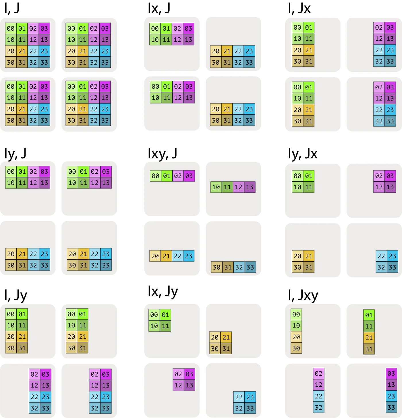
Here $A[I_{XY}, J]$ means that we treat the X and Y mesh axes as a larger flattened dimension and partition the I named axis across all the devices. The order of the multiple mesh-axis subscripts matters, as it specifies the traversal order of the partitioning across the grid.

Lastly, note that we cannot have multiple named axes sharded along the same mesh dimension. e.g. $A[I_X, J_X]$ is a nonsensical, forbidden sharding. Once a mesh dimension has been used to shard one dimension of an array, it is in a sense “spent”.

Pop Quiz: Let A be an array with shape int8[128, 2048], sharding $A[I_{XY}, J]$, and mesh Mesh({‘X': 2, ‘Y': 8, ‘Z': 2}) (so 32 devices total). How much memory does A use per device? How much total memory does A use across all devices?

Click here for the answer.

Answer: Our array A is sharded over X and and Y and replicated over Z, so per device it has shape int8[128 / (2 * 8), 2048] = int8[8, 2048], with size 8 * 2048 = 16,384 bytes. Because it’s replicated over Z, while within a Z-plane it’s fully sharded over X and Y, there’s one copy of it per Z-plane, and 2 such planes, so the total size (across all devices) is 128 * 2048 * 2 = 512kiB total.

A quick aside: how would we describe this in code?

JAX uses a named sharding syntax that very closely matches the abstract syntax we describe above. We’ll talk more about this in Section 10, but here’s a quick preview. You can play with this in a Google Colab here and profile the result to see how JAX handles different shardings. This snippet does 3 things:

1. Creates a jax.Mesh that maps our 4 TPUs into a 2x2 grid with names ‘X’ and ‘Y’ assigned to the two axes.
2. Creates matrices A and B where A is sharded along both its dimensions and B is sharded along the output dimension.
3. Compiles and performs a simple matrix multiplication that returns a sharded array.

import jax
import jax.numpy as jnp
import jax.sharding as shd

# Create our mesh! We're running on a TPU v2-8 4x2 slice with names 'X' and 'Y'.
assert len(jax.devices()) == 8
mesh = jax.make_mesh(axis_shapes=(4, 2), axis_names=('X', 'Y'))

# A little utility function to help define our sharding. A PartitionSpec is our
# sharding (a mapping from axes to names).
def P(*args):
  return shd.NamedSharding(mesh, shd.PartitionSpec(*args))

# We shard both A and B over the non-contracting dimension and A over the contracting dim.
A = jnp.zeros((8, 2048), dtype=jnp.bfloat16, device=P('X', 'Y'))
B = jnp.zeros((2048, 8192), dtype=jnp.bfloat16, device=P(None, 'Y'))

# We can perform a matmul on these sharded arrays! out_shardings tells us how we want
# the output to be sharded. JAX/XLA handles the rest of the sharding for us.
compiled = jax.jit(lambda A, B: jnp.einsum('BD,DF->BF', A, B), out_shardings=P('X', 'Y')).lower(A, B).compile()
y = compiled(A, B)

The cool thing about JAX is that these arrays behave as if they’re unsharded! B.shape will tell us the global or logical shape (2048, 8192). We have to actually look at B.addressable_shards to see how it’s locally sharded. We can perform operations on these arrays and JAX will attempt to figure out how to broadcast or reshape them to perform the operations. For instance, in the above example, the local shape of A is [4, 1024] and for B is [2048, 4096]. JAX/XLA will automatically add communication across these arrays as necessary to perform the final multiplication.

Computation With Sharded Arrays

If you have an array of data that’s distributed across many devices and wish to perform mathematical operations on it, what are the overheads associated with sharding both the data and the computation?

Obviously, this depends on the computation involved.

• For elementwise operations, there is no overhead for operating on a distributed array.
• When we wish to perform operations across elements resident on many devices, things get complicated. Thankfully, for most machine learning nearly all computation takes place in the form of matrix multiplications, and they are relatively simple to analyze.

When we think about sharded matrix multiplications, there are generally 4 cases we need to consider:

1. Case 1: neither input is sharded along the contracting dimension. We can multiply local shards without any communication.
2. Case 2: one input has a sharded contracting dimension. We typically “AllGather” the sharded input along the contracting dimension.
3. Case 3: both inputs are sharded along the contracting dimension. We can multiply the local shards, then “AllReduce” the result.
4. Case 4: both inputs have a non-contracting dimension sharded along the same axis. We cannot proceed without AllGathering one of the two inputs first.

You can think of these as rules that simply need to be followed, but it’s also valuable to understand why these rules hold and how expensive they are. We’ll go through each one of these in detail now.

You can also think of these rules in terms of “block matrix multiplcation”.

First let’s recall the concept of a “block matrix”, or a nested matrix of matrices:

\[\begin{equation} \begin{pmatrix} a_{00} & a_{01} & a_{02} & a_{03} \\ a_{10} & a_{11} & a_{12} & a_{13} \\ a_{20} & a_{21} & a_{22} & a_{23} \\ a_{30} & a_{31} & a_{32} & a_{33} \end{pmatrix} = \left( \begin{matrix} \begin{bmatrix} a_{00} & a_{01} \\ a_{10} & a_{11} \end{bmatrix} \\ \begin{bmatrix} a_{20} & a_{21} \\ a_{30} & a_{31} \end{bmatrix} \end{matrix} \begin{matrix} \begin{bmatrix} a_{02} & a_{03} \\ a_{12} & a_{13} \end{bmatrix} \\ \begin{bmatrix} a_{22} & a_{23} \\ a_{32} & a_{33} \end{bmatrix} \end{matrix} \right) = \begin{pmatrix} \mathbf{A_{00}} & \mathbf{A_{01}} \\ \mathbf{A_{10}} & \mathbf{A_{11}} \end{pmatrix} \end{equation}\]

Matrix multiplication has the nice property that when the matrix multiplicands are written in terms of blocks, the product can be written in terms of block matmuls following the standard rule:

\[\begin{equation} \begin{pmatrix} A_{00} & A_{01} \\ A_{10} & A_{11} \end{pmatrix} \cdot \begin{pmatrix} B_{00} & B_{01} \\ B_{10} & B_{11} \end{pmatrix} = \begin{pmatrix} A_{00}B_{00} + A_{01}B_{10} & A_{00}B_{01} + A_{01}B_{11} \\ A_{10}B_{00} + A_{11}B_{10} & A_{10}B_{01} + A_{11}B_{11} \end{pmatrix} \end{equation}\]

What this means is that implementing distributed matrix multiplications reduces down to moving these sharded blocks over the network, performing local matrix multiplications on the blocks, and summing their results. The question then is what communication to add, and how expensive it is.

Case 1: neither multiplicand has a sharded contracting dimension

Lemma: when multiplying partitioned tensors, the computation is valid and the output follows the sharding of the inputs unless the contracting dimension is sharded or both tensors have a non-contracting dimension sharded along the same axis. For example, this works fine

\[\begin{equation*} \mathbf{A}[I_X, J] \cdot \mathbf{B}[J, K_Y] \rightarrow \mathbf{C}[I_X, K_Y] \end{equation*}\]

with no communication whatsoever, and results in a tensor sharded across both the X and Y hardware dimensions. Try to think about why this is. Basically, the computation is independent of the sharding, since each batch entry has some local chunk of the axis being contracted that it can multiply and reduce. Any of these cases work fine and follow this rule:

\[\begin{align*} \mathbf{A}[I, J] \cdot \mathbf{B}[J, K] \rightarrow &\ \mathbf{C}[I, K] \\ \mathbf{A}[I_X, J] \cdot \mathbf{B}[J, K] \rightarrow &\ \mathbf{C}[I_X, K]\\ \mathbf{A}[I, J] \cdot \mathbf{B}[J, K_Y] \rightarrow &\ \mathbf{C}[I, K_Y]\\ \mathbf{A}[I_X, J] \cdot \mathbf{B}[J, K_Y] \rightarrow &\ \mathbf{C}[I_X, K_Y] \end{align*}\]

Because neither A nor B has a sharded contracting dimension J, we can simply perform the local block matrix multiplies of the inputs and the results will already be sharded according to the desired output shardings. When both multiplicands have non-contracting dimensions sharded along the same axis, this is no longer true (see the invalid shardings section for details).

Case 2: one multiplicand has a sharded contracting dimension

Let us consider the simple case of the distributed matrix multiply of A sharded in the contracting J dimension against a fully replicated B:

\[\mathbf{A}[I, J_X] \cdot \mathbf{B}[J, K] \rightarrow \mathbf{C}[I, K]\]

We cannot simply perform local matrix multiplies of the local A, B blocks against one another as we’re missing the full data from the contracting axis of A. Typically, we first “AllGather” the shards of A together locally, and only then multiply against B:

\[\textbf{AllGather}_X[I, J_X] \rightarrow \mathbf{A}[I, J]\] \[\mathbf{A}[I, J] \cdot \mathbf{B}[J, K] \rightarrow \mathbf{C}[I, K]\]

AllGathers remove sharding along an axis and reassembles the shards spread across devices onto each device along that axis. Using the notation above, an AllGather removes a subscript from a set of axes, e.g.

\[\textbf{AllGather}_{XY}(A[I_{XY}, J]) \rightarrow A[I, J]\]

We also don’t have to remove all subscripts for a given dimension, e.g. \(A[I_{XY}, J] \rightarrow A[I_Y, J]\) is also an AllGather, just over only a single axis.

Note that we may also wish to use an AllGather to remove non-contracting dimension sharding, for instance the matrix multiply:

\[A[I_X, J] \cdot B[J, K] \rightarrow C[I, K]\]

We would similarly AllGather along X to remove the output sharding, however in this case we have the freedom of doing so before or after the matrix multiply, unlike in the case of AllGathering the contracting dimension, where we are forced to do so before performing the matrix multiply.

How is an AllGather actually performed? To perform an AllGather along a single axis, we need to pass all the shards around the axis until every device has a copy. Figure 1 shows an example. Each of the 8 devices starts with 1 / 8th of the array and ends up with all copies. One efficient way to do this is to have each device pass its shard around the sharding dimension ring, either in one direction or both directions. If we do one direction, it takes \(N - 1\) hops of size \(\text{total size} / N\) per-link, otherwise we have $\lceil \frac{N}{2} \rceil$ hops of size \(2 \cdot \text{total size} / N\) per link.

How long does this take? Let’s take the bidirectional AllGather and calculate how long it takes. Let \(V\) be the number of bytes in the array, and \(\lvert X\rvert\) be the number of shards on the contracting dimension. Then from the above diagram, each hop sends $V / \lvert X\rvert$ bytes in each direction, so each hop takes

\[T_{hop} = \frac{2 \cdot V}{|X| \cdot W_{ICI}}\]

where \(W_\text{ICI}\) is the bidirectional ICI bandwidth. We need to send a total of $\lvert X\rvert / 2$ hops to reach every TPUtechnically, $\lceil | X | / 2 \rceil$, so the total reduction takes

\[T_{total} = \frac{2 \cdot V \cdot |X|}{2 \cdot |X| \cdot W_\text{ICI}}\] \[T_{total} = \frac{V}{W_\text{ICI}}\]

Note that this doesn’t depend on \(\lvert X\rvert\)! That’s kind of striking, because it means even though our TPUs are only locally connected, the locality of the connections doesn’t matter. We’re just bottlenecked by the speed of each link.

Takeaway: when performing an AllGather (or a ReduceScatter or AllReduce) in a throughput-bound regime, the actual communication time depends only on the size of the array and the available bandwidth, not the number of devices over which our array is sharded!

A note on ICI latency: Each hop over an ICI link has some intrinsic overhead regardless of the data volume. This is typically around 1us. This means when our array \(A\) is very small and each hop takes less than 1us, we can enter a “latency-bound” regime where the calculation does depend on \(\lvert X \rvert\).

For the full details, click here.

Let \(T_\text{min}\) be the minimum time for a single hop. Then

\[T_{hop} = \max \left[ T_{min}, \frac{2 \cdot V}{|X| \cdot W_\text{ICI}} \right]\] \[T_{total} = \max \left[ \frac{T_{min} \cdot |X|}{2}, \frac{V}{W_\text{ICI}} \right]\]

since we perform \(\lvert X \rvert / 2\) hops. For large reductions or gathers, we’re solidly bandwidth bound. We’re sending so much data that the overhead of each hop is essentially negligible. But for small arrays (e.g. when sampling from a model), this isn’t negligible, and the ICI bandwidth isn’t relevant. We’re bound purely by latency. Another way to put this is that given a particular TPU, e.g. TPU v5e with 4.5e10 unidirectional ICI bandwidth, sending any buffer under 4.5e10 * 1e-6 = 45kB will be latency bound.

What happens when we AllGather over multiple axes? When we gather over multiple axes, we have multiple dimensions of ICI over which to perform the gather. For instance, AllGather_XY([B, D_XY]) operates over two hardware mesh axes. This increases the available bandwidth by a factor of \(n_\text{axes}\).

For the full details, click here.

In general we have

\[T_{total} = \max \left[ \frac{T_{min} \cdot \sum_{i} |X_i|}{2}, \frac{V}{W_\text{ICI} \cdot n_\text{axes}} \right]\]

where \(\sum_i \lvert X_i \rvert / 2\) is the length of the longest path in the TPU mesh.

Pop Quiz 2 [AllGather time]: Using the numbers from Part 2, how long does it take to perform the AllGather_Y([E_Y, F]) → [E, F] on a TPUv5e with a 2D mesh {'X': 8, 'Y': 4}, \(E = 2048\), \(F = 8192\) in bfloat16? What about with \(E=256, F=256\)?

Click here for the answer.

Answer: Let’s start by calculating some basic quantities:

1) TPU v5e has 9e10 bytes/s of bidirectional ICI bandwidth for each of its 2 axes.
2) In bfloat16 for (a), we have $A[E_Y, F]$ so each device holds an array of shape bfloat16[512, 8192] which has 512 * 8192 * 2 = 8.4MB. The total array has size 2048 * 8192 * 2 = 34MB.

For part (1), for a first approximation, we can use the formula above. Since we’re performing the AllGather over one axis, we have $T_{\text{comms}} = 34e6\text{ bytes }/ (9e10\text{ bytes / s } * 1) = 377\mu s$. To check that we’re not latency-bound, we know over an axis of size 4, we’ll have at most 3 hops, so our latency bound is something like 3us, so we’re not close. However, TPU v5e only has a wraparound connection when one axis has size 16, so here we actually can’t do a fully bidirectional AllGather. We have to do 3 hops for data from the edges to reach the other edge, so in theory we have more like $T_{\text{comms}} = 3 * 8.4e6 / 4.5e10 = 560\mu s$. Here’s an actual profile from this Colab, which shows $680 \mu s$, which is reasonable since we’re likely not getting 100% of the theoretical bandwidth! For part (2) each shard has size 64 * 256 * 2 = 32kB. 32e3 / 4.5e10 = 0.7us, so we’re latency bound. Since we have 3 hops, this will take roughly 3 * 1us = 3us. In practice, it’s closer to 8us.

Case 3: both multiplicands have sharded contracting dimensions

The third fundamental case is when both multiplicands are sharded on their contracting dimensions, along the same mesh axis:

\[\textbf{A}[I, J_X] \cdot \textbf{B}[J_X, K] \rightarrow C[I, K]\]

In this case the local sharded block matrix multiplies are at least possible to perform, since they will share the same sets of contracting indices. But each product will only represent a partial sum of the full desired product, and each device along the X dimension will be left with different partial sums of this final desired product. This is so common that we extend our notation to explicitly mark this condition:

\[\textbf{A}[I, J_X] \cdot_\text{LOCAL} \textbf{B}[J_X, K] \rightarrow C[I, K] \{\ U_X \}\]

The notation { U_X } reads “unreduced along X mesh axis” and refers to this status of the operation being “incomplete” in a sense, in that it will only be finished pending a final sum. The *local syntax means we perform the local sum but leave the result unreduced.

This can be seen as the following result about matrix multiplications and outer products:

\[A \cdot B = \sum_{i=1}^{P} \underbrace{A_{:,i} \otimes B_{i,:}}_{\in \mathbb{R}^{n \times m}}\]

where ⊗ is the outer product. Thus, if TPU i on axis X has the ith column of A, and the ith row of B, we can do a local matrix multiplication to obtain \(A_{:,i} \otimes B_{i,:} \in \mathbb{R}_{n\times m}\). This matrix has, in each entry, the ith term of the sum that A • B has at that entry. We still need to perform that sum over P, which we sharded over mesh axis X, to obtain the full A • B. This works the same way if we write A and B by blocks (i.e. shards), and then sum over each resulting shard of the result.

We can perform this summation using a full AllReduce across the X axis to remedy this:

\[\begin{align*} A[I, J_X] \cdot_\text{LOCAL} B[J_X, K] \rightarrow &\ C[I, K] \{ U_X \} \\ \textbf{AllReduce}_X C[I, K] \{ U_X \} \rightarrow &\ C[I, K] \end{align*}\]

AllReduce removes partial sums, resulting in each device along the axis having the same fully-summed value. AllReduce is the second of several key communications we’ll discuss in this section, the first being the AllGather, and the others being ReduceScatter and AllToAll. An AllReduce takes an array with an unreduced (partially summed) axis and performs the sum by passing those shards around the unreduced axis and accumulating the result. The signature is

\[\textbf{AllReduce}_Y A[I_X, J] \{U_Y\} \rightarrow A[I_X, J]\]

This means it simply removes the $\{U_Y\}$ suffix but otherwise leaves the result unchanged.

How expensive is an AllReduce? One mental model for how an AllReduce is performed is that every device sends its shard to its neighbors, and sums up all the shards that it receives. Clearly, this is more expensive than an AllGather because each “shard” has the same shape as the full array. Generally, an AllReduce is twice as expensive as an AllGather. One way to see this is to note that an AllReduce can be expressed as a composition of two other primitives: a ReduceScatter and an AllGather. Like an AllReduce, a ReduceScatter resolves partial sums on an array but results in an output ‘scattered’ or partitioned along a given dimension. AllGather collects all those pieces and ‘unpartitions/unshards/replicates’ the logical axis along that physical axis.

\[\begin{align*} \textbf{ReduceScatter}_{Y,J} : A[I_X,J] \{U_Y\} \rightarrow &\ A[I_X, J_Y] \\ \textbf{AllGather}_Y : A[I_X, J_Y] \rightarrow &\ A[I_X, J] \end{align*}\]

What about a ReduceScatter? Just as the AllReduce removes a subscript ($F_Y \to F$ above), a ReduceScatter sums an unreduced/partially summed array and then scatters (shards) a different logical axis along the same mesh axis. $[F]\{U_Y\} \to [F_Y]$. The animation shows how this is done: note that it’s very similar to an AllGather but instead of retaining each shard, we sum them together. Thus, its latency is roughly the same, excluding the time taken to perform the reduction.

The communication time for each hope is simply the per-shard bytes \(V\) divided by the bandwidth, as it was for an AllGather, so we have

\[T_{\text{comms per AllGather or ReduceScatter}} = \frac{V}{W_\text{ICI}}\] \[T_{\text{comms per AllReduce}} = 2 \cdot \frac{V}{W_\text{ICI}}\]

where \(W_\text{ICI}\) is the bidirectional bandwidth, so long as we have a full ring to reduce over.

Case 4: both multiplicands have a non-contracting dimension sharded along the same axis

Each mesh dimension can appear at most once when sharding a tensor. Performing the above rules can sometimes lead to a situation where this rule is violated, such as:

\[A[I_X, J] \cdot B[J, K_X] \rightarrow C[I_X, K_X]\]

This is invalid because a given shard, say i, along dimension X, would have the (i, i)th shard of C, that is, a diagonal entry. There is not enough information among all shards, then, to recover anything but the diagonal entries of the result, so we cannot allow this sharding.

The way to resolve this is to AllGather some of the dimensions. Here we have two choices:

\[\begin{align*} \textbf{AllGather}_X A[I_X, J] \rightarrow &\ A[I, J] \\ A[I, J] \cdot B[J, K_X] \rightarrow &\ C[I, K_X] \end{align*}\]

or

\[\begin{align*} \textbf{AllGather}_X B[J, K_X] \rightarrow &\ B[J, K] \\ A[I_X, J] \cdot B[J, K] \rightarrow &\ C[I_X, K] \end{align*}\]

In either case, the result will only mention X once in its shape. Which one we pick will be based on what sharding the following operations need.

A Deeper Dive into TPU Communicaton Primitives

The previous 4 cases have introduced several “core communication primitives” used to perform sharded matrix multiplications:

1. AllGather: removes a subscript from a sharding, gathering the shards.
2. ReduceScatter: removes an “un-reduced” suffix from an array by summing shards over that axis, leaving the array sharded over a second axis.
3. AllReduce: removes an “un-reduced” suffix, leaving the array unsharded along that axis.

There’s one more core communication primitive to mention that arises in the case of Mixture of Experts (MoE) models and other computations: the AllToAll.

Our final communication primitive: the AllToAll

A final fundamental collective which does not occur naturally when considering sharded matrix multiplies, but which comes up constantly in practice, is the AllToAll collective, or more precisely the special case of a sharded transposition or resharding operation. e.g.

\[\textbf{AllToAll}_{X, J} A[I_X, J] \rightarrow A[I, J_X]\]

AllToAlls are typically required to rearrange sharded layouts between different regions of a sharded computation that don’t have compatible layout schemes. They arise naturally when considering sharded mixture-of-experts models. You can think of an AllToAll as moving a subscript from one axis to another. Because an all to all doesn’t need to replicate all of the data of each shard across the ring, it’s actually cheaper than an allgather (by a factor of ¼).For even-sized bidirectional rings, each device will send $(N/2 + (N/2-1) + … + 1)$ chunks right and $((N/2-1) + … + 1)$ chunks left $= 0.5 \cdot (N / 2) \cdot (N/2 + 1) + 0.5 \cdot (N / 2) \cdot (N/2 - 1) = N^2/4$. The size of each chunk (aka shard of a shard) is $\text{bytes} / N^2$ so the per-device cost is $(\text{bytes} / N^2) \cdot N^2 / 4 = \text{bytes} / 4$. This result scales across all devices as the total bandwidth scales with device number.

More about the ReduceScatter

ReduceScatter is a more fundamental operation than it first appears, as it is actually the derivative of an AllGather, and vice versa. i.e. if in the forward pass we have:

\[\textbf{AllGather}_X A[I_X] \rightarrow A[I]\]

Then we ReduceScatter the reverse-mode derivatives A’ (which will in general be different on each shard) to derive the sharded A’:

\[\textbf{ReduceScatter}_X A'[I] \{ U_X \} \rightarrow A'[I_X]\]

Likewise, \(\text{ReduceScatter}_X(A[I] \{U_X\}) \to A[I_X])\) in the forward pass implies \(\text{AllGather}_{X}(A'[I_X]) \to A'[I]\) in the backwards pass.

Turning an AllReduce into an AllGather and ReduceScatter also has the convenient property that we can defer the final AllGather until some later moment. also has the convenient property that Very commonly we’d rather not pay the cost of reassembling the full matrix product replicated across the devices. Rather we’d like to preserve a sharded state even in this case of combining two multiplicands with sharded contracting dimensions:

\[A[I, J_X] \cdot B[J_X, K] \rightarrow C[I, K_X]\]

In this case, we can also perform a ReduceScatter instead of an AllReduce, and then optionally perform the AllGather at some later time, i.e.

\[\begin{align*} A[I, J_X] \cdot_{LOCAL} B[J_X, K] \rightarrow &\ C[I, K] \{ U_X \} \\ \textbf{ReduceScatter}_{X,K} C[I, K] \{ U_X \} \rightarrow &\ C[I, K_X] \end{align*}\]

Note that ReduceScatter introduces a sharded dimension, and so has a natural freedom to shard along either the I or K named dimensions in this case. We generally need to choose which named dimension to introduce a new sharding to when using a ReduceScatter (though the choice is usually forced by the larger modeling context). This is why we use the syntax ReduceScatter_X,K to specify the axis to shard.

What Have We Learned?

• The sharding of an array is specified by a Mesh that names the physical, hardware axes of our TPU mesh and a Sharding that assigns mesh axis names to the logical axes of the array.

• For example, A[I_XY, J] describes an abstract array A with its first dimension sharded along two mesh axes X and Y. Combined with Mesh(mesh_shape=(4, 8), axis_names=(‘X’, ‘Y’)) or the abbreviated Mesh({‘X’: 4, ‘Y’: 8}), this tells us our array is sharded 32 ways along the first dimension.

• Arithmetic with sharded arrays works exactly like with unsharded arrays unless you perform a contracting along a sharded axis. In that case, we have to introduce some communication.

• TPUs use roughly 4 core communication primitives:
  1. AllGather: $[A_X, B] \to [A, B]$
  2. ReduceScatter: $[A, B] \{U_X\} \to [A, B_X]$
  3. AllToAll: $[A, B_X] \to [A_X, B]$
  4. AllReduce: $[A_X, B]\{U_Y\} \to [A_X, B]$ (technically not a primitive since it combines a ReduceScatter + AllGather)

• The cost and latency of each of these operations doesn’t depend on the size of the axis (as long as they’re bandwidth bound), but only on the size of the input arrays and the bandwidth of the link.

\[T_{\text{comm per AllGather or ReduceScatter}} = \frac{\text{Data volume}}{\text{bandwidth}} \cdot \frac{\text{Axis} - 1}{\text{Axis}} \longrightarrow \frac{\text{Data volume}}{\text{bandwidth (bidirectional)}}\]

• An AllReduce is composed of a ReduceScatter followed by an AllGather, and thus has 2x the above cost. An AllToAll only has to pass shards part-way around the ring and is thus ¼ the cost of an AllGather. Here’s a summary:

Operation	Description	Syntax	Runtime
AllGather	Gathers all the shards of a sharded array along an axis, removing a subscript.	$[A_X, B] \to [A, B]$	bytes / (bidirectional ICI bandwidth * num_axes)
ReduceScatter	Sums a partially summed array along an axis and shards it along another axis (adding a subscript).	$[A, B] \{U_X\} \to [A_X, B]$	Same as AllGather
AllReduce	Sums a partially summed array along an axis. Removes a { Ux }. Combines an AllGather and ReduceScatter.	$[A_X, B]\{U_Y\} \to [A_X, B]$	2 * AllGather
AllToAll	Gathers (replicates) an axis and shards a different dimension along the same axis.	$[A, B_X] \to [A_X, B]$	AllGather / 4 for a bidirectional ring

• Note that we use the bidirectional bandwidth above, while the numbers reported in Section (1) are unidirectional.

• When performing sharded matmuls, we consider 3 main cases:

  1. Neither array is sharded along the contracting dimension: no communication is needed.
  2. One array is sharded along the contracting dimension (or the contracting dimensions are sharded along different axes): we AllGather one of the inputs before performing the operation.
  3. Both arrays are identically sharded along the contracting dimension: we multiply the shards locally then perform an AllReduce or ReduceScatter.

Some Problems to Work

Here are some instructive problems based on content in this section. We won’t include all answers at the moment but we’ll write up more answers as we can.

Question 1 [replicated sharding]: An array is sharded $A[I_X, J, K, \ldots]$ (i.e., only sharded across $X$), with a mesh Mesh({'X': 4, 'Y': 8, 'Z': 2}). What is the ratio of the total number of bytes taken up by $A$ across all chips to the size of one copy of the array?

Click here for the answer.

Our array is only sharded along X, which has size 4, so effectively each shard has size $[I / 4, J, K, \ldots] = \text{sizeof}(A) / 4$. Since our array is replicated across Y and Z, the total size is $Y \cdot Z \cdot \text{sizeof}(A)$, so the ratio of total size to single chip size is $Y \cdot Z \cdot \text{sizeof}(A) / \text{sizeof}(A) = 16$.

Question 2 [AllGather latency]: How long should $\text{AllGather}_X([B_X, D_Y])$ take on a TPUv4p 4x4x4 slice with mesh Mesh({'X': 4, 'Y': 4, 'Z': 4}) if $B=1024$ and $D=4096$ in bfloat16? How about $\text{AllGather}_Y([B_X, D_Y])$? How about \(\text{AllGather}_{XY}([B_X, D_Y])\)? How about \(\text{AllGather}_Z([B_X, D_Y]\{U_Z\})\)?

Click here for the answer.

1. Because we’re just gathering over one axis and the other is sharded, we’re effectively gathering $\frac{2BD}{Y}$ bytes over 1 axis. Since our ICI bandwidth for TPU v4p is 9e10 bytes/second bidirectional, this will take $\frac{2BD}{9e10 \cdot Y} = \frac{2 \cdot 1024 \cdot 4096}{9e10 \cdot 4} = 23 \mu s$. We have a full wraparound on the 4 axes so we can use the full bidirectional bandwidth.

2. We’re gathering along a wraparound axis of size $Y=4$, the total data we have to move is $2BD/Y$ bytes, and the bidirectional bandwidth on v4p is 9e10 bytes/second, so once more we get $\frac{2BD}{9e10 \cdot Y} = 23 \mu s$.

3. We use the multi-axis equation, and find that \(T_{\text{total}} = \max\{4 \cdot T_{\text{min}}, \frac{2BD}{2 \cdot W_{\text{ICI}}}\}\). The per-hop latency in TPU v5e is $\frac{1}{2}\mu s$, so the left operand is $2 \mu s$. The right operand is $\frac{2 \cdot 1024 \cdot 4096}{1.8e11}$ seconds, or $46 \mu s$, so we’re throughput bound, not latency bound.

4. The result of this operation has shape $[B_X, D_Y]$, so the number of bytes in the array each machine will hold is $\frac{2BD}{XY}$. We have wraparound links for the $Z$ axis since it’s a multiple of 4 in TPU v5e, so we get a bidirectional bandwidth of 9e10 bytes / second. Thus this operation takes time $\frac{2 \cdot 1024 \cdot 4096}{16 \cdot 9e10}$ seconds, or $5.8 \mu s$.

Question 3 [latency-bound AllGather]: Let’s say we’re performing an $\text{AllGather}_X([B_X])$ but $B$ is very small (say 128). How long should this take on a TPUv4p 4x4x4 slice with mesh Mesh({'X': 4, 'Y': 4, 'Z': 4}) in bfloat16? Hint: you’re probably latency bound.

Click here for the answer.

Our array in bfloat16 uses only 256 bytes total, and only 64 per device. Since we have an axis of size 4 on a TPU v4p, we have a wraparound link, so we can do the AllGather by sending half the bytes in each direction, meaning only 32 bytes in each direction. With 4.5e10 of unidirectional bandwidth, each hop would take roughly 32 / 4.5e10 ~ 0, so we’re definitely latency bound. Counting the number of hops, we can do the full gather in only 2 hops, so roughly 2us a good estimate.

Question 4 [matmul strategies]: To perform $A[B, D] \cdot_D B[D_X, F] \to C[B, F]$, instead of performing $\text{AllGather}_X(B[D_X, F])$ and multiplying the fully replicated matrices (as we suggest in this doc), you could multiply the local shards resulting in $C[B, F]\{U_X\}$ and then $\text{AllReduce}_X(C[B, F] \{ U_X\})$. How many FLOPs and comms does each of these perform? Which is better and why?

Click here for the answer.

Since we’re multiplying our sharded matrices, the total FLOPs performed is much smaller than with the AllGather. We do \(2\cdot B\cdot D\cdot F / X\) FLOPs and the resulting AllReduce communicates \(2 \cdot 2 \cdot B \cdot F\) bytes in bfloat16. Thus, our total time for Strategy 1 (no AllGather, just an AllReduce later on) is roughly

\[T_\text{total} = \max\left(\frac{2BDF}{X * C}, \frac{4BF}{W_{ICI}}\right)\]

where \(C\) is our accelerator FLOPs/s. The baseline does half as many comms and X times more FLOPs since the computation isn’t sharded. This means we do \(2\cdot B\cdot D\cdot F\) FLOPs and send \(2\cdot B\cdot D\) bytes (since AllGather is half as expensive). So for Strategy 2 we have

\[T_\text{total} = \max\left(\frac{2BDF}{C}, \frac{2BD}{W_{ICI}}\right)\]

The question is: which of these is bigger? Strategy (1) is compute bound when \(D / (X * C) > 2 / W<_\text{ICI}\), or when \(D / 2X > C / W_\text{ICI} \approx 2550 \rightarrow X < D / (2 * 2550)\). We might reasonably expect \(D \approx 8k\), so this would mean roughly \(X < 2\) which is unlikely. So we’re basically always comms bound in the first case. In the second case (baseline), we’re comms bound when \(F < C / W_\text{ICI} = 2550\) (which is rarely true), so we’re generally compute-bound. Thus, the question of whether strategy (1) is better becomes whether

\[T_\text{comms for Strategy 1} < T_\text{math for strategy 2} \Leftrightarrow \frac{4BF}{W_{ICI}} < \frac{2BDF}{C}\]

This is true when \(2 / W_\text{ICI} < D / C\), or when \(D > 2 * 2550 = 5100\), which is usually true for large models. So this alternative strategy is typically better for large models.

Why don’t we always do this? Well, in practice we may do this sometimes, but it’s typically rare to have the contracting dimension of one of the inputs to a matmul sharded along a axis that the other input isn’t sharded over. For instance, if we’re doing FSDP (explained in Section 5), we’ll sharded our parameters over the data dimension but our activations will also be sharded along data. So in this sense this doesn’t show up much.

Question 5 [minimum latency]: Let’s say I want to do a matmul $A[B, D] \cdot_D B[D, F] \to C[B, F]$ on a TPUv5p 4x4x4 with the lowest possible latency. How should my inputs be sharded? What is the total FLOPs and comms time?

Question 6: Let’s say we want to perform $A[I_X, J_Y] \cdot_J B[J_Y, K] \to C[I_X, K]$ on TPUv5e 4x4. What communication do we perform? How much time is spent on communication vs. computation?

• What about $A[I_X, J] \cdot_J B[J_X, K_Y] \to C[I_X, K_Y]$? This is the most standard setting for training where we combine data, tensor, and zero sharding.
• What about $A[I_X, J] \cdot_J B[J, K_Y] \to C[I_X, K_Y]$? This is standard for inference, where do pure tensor parallelism (+data).

Question 7: A typical Transformer block has two matrices $B[D, F]$ and $C[F, D]$ where $F \gg D$. With a batch size B, the whole block is \(C \cdot B \cdot x\) with \(x[B, D]\). Let’s pick \(D=8192\), \(F=32768\), and \(B=128\) and assume everything is in bfloat16. Assume we’re running on a TPUv5e 2x2 slice but assume each TPU only has 300MB of free memory. How should B, C, and the output be sharded to stay below the memory limit while minimizing overall time? How much time is spent on comms and FLOPs?

Question 8 [challenge]: Using the short code snippet above as a template, allocate a sharded array and benchmark each of the 4 main communication primitives (AllGather, AllReduce, ReduceScatter, and AllToAll) using pmap or shard_map. You will want to use jax.lax.all_gather, jax.lax.psum, jax.lax.psum_scatter, and jax.lax.all_to_all. Do you understand the semantics of these functions? How long do they take?

Question 9 [another strategy for sharded matmuls?]: Above we claimed that when only one input to a matmul is sharded along its contracting dimension, we should AllGather the sharded matrix and perform the resulting contracting locally. Another strategy you might think of is to perform the sharded matmul and then AllReduce the result (as if both inputs were sharded along the contracting dimension), i.e. $A[I, J_X] *_J B[J, K] \to C[I, K]$ by way of

1. $C[I, K] \{ U_X \} = A[I, J_X] \cdot B[J_X, K]$
2. $C[I, K] = \text{AllReduce}(C[I, K] \{ U_X\})$

Answer the following:

1. Explicitly write out this algorithm for matrices $A[N, M]$ and $B[M, K]$, using indices to show exactly what computation is done on what device. Assume $A$ is sharded as $A[I, J_X]$ across ND devices, and you want your output to be replicated across all devices.
2. Now suppose you are ok with the final result not being replicated on each device, but instead sharded (across either the N or K dimension). How would the algorithm above change?
3. Looking purely at the communication cost of the strategy above (in part (b), not (a)), how does this communication cost compare to the communication cost of the algorithm in which we first AllGather A and then do the matmul?

Click here for the answer.

1. First compute the outer products, storing the result in \(O[N, K]: o_{kj} = \sum_i a_{ik} b_{ji}\). Note that the repeated index is not the one being contracted, as we are doing an outer product. Here the sum ranges across the set of i values stored on the particular device we are using. So, for example, if we have a contracting axis of size 16, and 4 devices, then on device 0, i would range from {0, 1, 2, 3}; on device 1, i would range from {4, 5, 6, 7}; on device 2, i would range from {8, 9, 10, 11}; and on device 3, i would range from {12, 13, 14, 15}. Then AllReduce the partial-sums of $O[N, K]$ which live on each device, to form the full O[N x K].
2. Instead of doing an AllReduce in step 2, we could get away with a cheaper ReduceScatter, along either axis: $[N, K] \{ U_X \} \to [N_X, K]$ or $[N, K] \{ U_X \} \to [N, K_X]$.
3. As described in the main text above, the cost of doing an AllGather (when we are throughput-bound) is the same as that of a ReduceScatter; it is simply given by the size of the full matrix we are processing. So in the gather-then-matmul algorithm, this scales as $NM$ (since we are $\text{AllGather}$-ing $A$); in the matmul-then-reduce-scatter algorithm, this scales as NK (since we are reduce-scattering $O$). So the communication cost ratio of the two algorithms is M/K.

Question 10: Fun with AllToAll: In the table above, it was noted that the time to perform an AllToAll is a factor of 4 lower than the time to perform an AllGather or ReduceScatter (in the regime where we are throughput-bound). In this problem we will see where that factor of 4 comes from, and also see how this factor would change if we only had single-direction ICI links, rather than bidirectional ICI links.

1. Let’s start with the single-direction case first. Imagine we have D devices in a ring topology, and If we are doing either an AllGather or a ReduceScatter, on an N x N matrix A which is sharded as $A[I_X, J]$ (say $D$ divides $N$ for simplicity). Describe the comms involved in these two collectives, and calculate the total number of scalars (floats or ints) which are transferred across a single ICI link during the entirety of this algorithm.
2. Now let’s think about an AllToAll, still in the single-directional ICI case. How is the algorithm different in this case than the all-gather case? Calculate the number of scalars that are transferred across a single ICI link in this algorithm.
3. You should have found that the ratio between your answers to part (a) and part (b) is a nice number. Explain where this factor comes from in simple terms.
4. Now let’s add bidirectional communication. How does this affect the total time needed in the all-gather case?
5. How does adding bidirectional communication affect the total time needed in the AllToAll case?
6. Now simply explain the ratio between AllGather time and AllToAll time in a bidirectional ring.

Click here for the answer.

(1) Solution: The process is simple: in each step of the algorithm, each device will send a single-shard “strip” of the matrix (totalling \(\frac{N}{D} \times N\) elements in size) to its nearest neighbor. This occurs \(D-1\) times, since each shard needs to be communicated to all of the devices except the one it starts out on. So in total, \(\frac{N^2(D-1)}{D}\) scalars are transferred by each device, i.e. flow across a single ICI link.

Answer: \(N^2 (1-\frac{1}{D})\), or simply \(N^2\) when \(D >> 1\).

(2) Solution: The key difference between an AllToAll and an AllGather, from the perspective of communications, is that in an AllToAll, the entirety of the shard that lives on a particular device does not need to be communicated to every other device. Imagine the shard stored on a particular device (call it device 0) is \([A, B, C, D]\) (here A,B,C,D are matrices and we are imagining a ring with 4 devices for illustration). Now the matrix \(A\) does not need to be communicated anywhere, the matrix \(B\) needs to end up on device 1; matrix \(C\) ends up on device 2; and matrix \(D\) ends up on device 3. So in the first step of the algorithm, we send \(B\), \(C\), and \(D\) to device 1; in the next step, device 1 sends \(C\) and \(D\) onwards to device 2; in the final step, device 2 sends just \(D\) on to device 3. The total number of parameters transferred in this case is \((\text{size of A/B/C/D}) * (3 + 2 + 1)\). The size of A/B/C/D is (in the general case now) \(\frac{N^2}{D^2}\), and again in the general case the \((3 + 2 + 1)\) term becomes \(((D-1) + (D-2) + … + 1)\), or \(\frac{(D)(D-1)}{2}\). So the total number of bytes transferred across a single ICI link is \(\frac{N^2(D-1)}{D \times 2}\).

Answer: \(\frac{N^2}{2}(1-\frac{1}{D})\), or simply \(\frac{N^2}{2}\) when \(D >> 1\).

(3) Solution: The factor is simply \(\frac{1}{2}\), i.e. an AllToAll is half as costly as an all-gather/ReduceScatter on a unidirectional ring topology. Looking over the derivations above, this ultimately came from the fact that in the all-gather case, we are transferring the same sized block each of \((D-1)\) times, i.e. we’re doing the sum \(\text{tiny block size} * (D + D + D + … + D)\), whereas in the AllToAll case, we’re doing the sum \(\text{tiny block size} * (D + D-1 + D-2 + … + 1)\). The factor of two thus essentially comes from the fact that \(1 + 2 + \ldots + n = n(n+1)/2\).

(4) Solution: The total number of scalars that any one link has to carry now reduces by a factor of 2, since in a bidirectional ring, each “sharded strip” can be sent two ways simultaneously.

(5) Solution: In this case, we win a factor of 4 compared to the unidirectional case. This is easiest to see by considering the fate of each of the size-(N2/D2) blocks in a single sharded strip, say the one which originates on device 0. Instead of (as in the unidirectional case) sending one of these blocks a distance of D-1, another block a distance D - 2, etc. all the way to 1, we now divide the strip into blocks which move right or left, moving a maximum distance of ceil(D/2). So the corresponding sum now becomes \(D/2 + D/2 - 1 + D/2 - 2 + … = D/2 \cdot (D/2-1)/2\), or \(D^2/8\) in the limit of large \(D\). Compare this to \(D^2/2\) in the unidirectional case, and we see that we’ve won a factor of 4.

(6) Solution: In a unidirectional ring, we saw that the AllToAll time was already twice as fast as the all-gather time; this comes from the fact that we don’t need to send our full strip to every single device. Then, when we added bidirectionality, we saw that it was a 4x win for AllToAll, and only a 2x win for all-gathers. Putting these ratios together, we get our sought after factor of 4.

That’s it for Part 3! For Part 4 (about Transformer math), click here!